Today we’re excited to announce NVIDIA DIGITS 5. DIGITS 5 comes with a number of new features, two of which are of particular interest for this post:
- a fully-integrated segmentation workflow, allowing you to create image segmentation datasets and visualize the output of a segmentation network, and
- the DIGITS model store, a public online repository from which you can download network descriptions and pre-trained models.
In this post I will explore the subject of image segmentation. I’ll use DIGITS 5 to teach a neural network to recognize and locate cars, pedestrians, road signs and a variety of other urban objects in synthetic images from the SYNTHIA dataset.
Figure 1 shows a preview of what you will learn to do in this post.

From Image Classification to Image Segmentation
Suppose you want to design image understanding software for self-driving cars. Chances are you’ve heard about Alexnet [1], GoogLeNet [2], VGG-16 [3] and other image classification neural network architectures, so you might want to start from there. Image classification is the process by which a computer program is able to tell you that a picture of a dog is a picture of a dog.
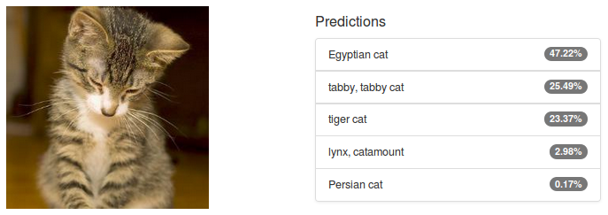
The output of an image classification model is a discrete probability distribution: one number between 0 and 1—a probability—for each class the model is trained to recognise. Figure 2 illustrates an example classification of an image of a cat using Alexnet in DIGITS. The result is spectacularly good: remember that Alexnet was trained on 1000 different classes of objects from categories including animals, musical instruments, vegetables, vehicles and many others. I find it humbling to see that with over 99% confidence, a machine is able to correctly classify the subject of the image as feline. I, for one, would be at a loss to tell whether that particular cat is an Egyptian, tabby or tiger cat.
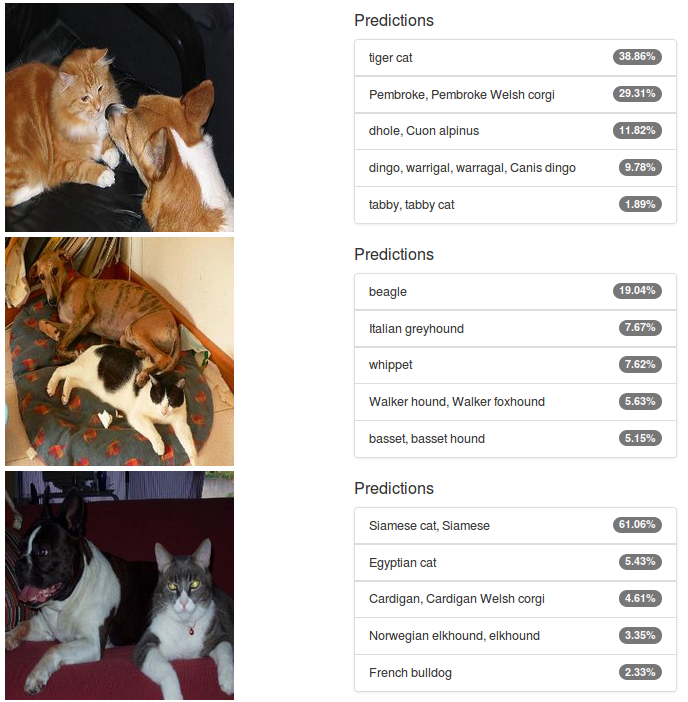
But what happens if you classify an image of a cat and a dog? Common sense might lead you to believe that the neural network would assign an equal share of the probability distribution to our two favorite pet species. Let’s try it: Figure 3 shows the outcome. There is a mix of cats and dogs in the predictions, but AlexNet doesn’t deliver the hoped-for 50/50 split. In the middle picture there are in fact no cats within the Top 5 predictions. This is disappointing, but on the other hand Alexnet was trained on a “small” world of 1.2 million images in which there is only ever one object to see, so one can’t reasonably expect it to perform well in the presence of multiple objects.
Another limitation of classification networks is their inability to tell the location of objects in images. Again, this is understandable, considering that they were not trained to do this, but this is nonetheless a major hindrance in computer vision: if a self-driving car is unable to determine the location of the road it will probably not travel a long way!
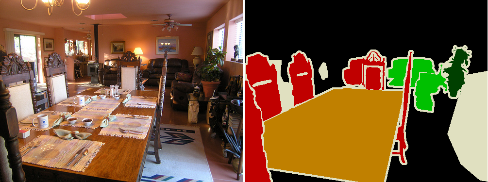
Image segmentation addresses some of these shortcomings. Instead of predicting a single probability distribution for the whole image, the image is divided into a number of blocks and each block is assigned its own probability distribution. In the most common embodiment, images are divided down to pixel level and each pixel is classified: for every pixel in the image, the network is trained to predict which class that particular pixel is part of. This allows the network to not only identify several object classes in each image, but also to determine the location of objects. Image segmentation typically generates a label image the same size as the input whose pixels are color-coded according to their classes. Figure 4 shows an example that segments four different classes in a single image: table, chair, sofa and potted-plant.
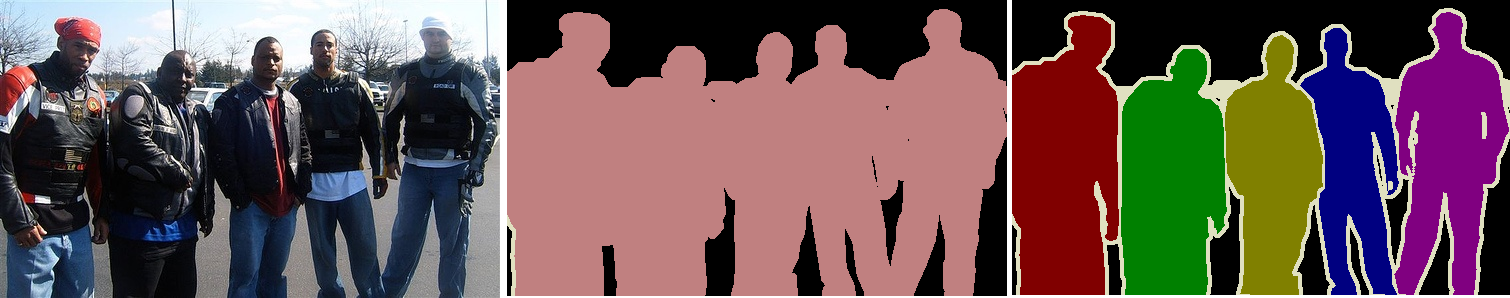
In a further refinement of image segmentation named Instance-aware Image Segmentation (IAIS) the network learns to identify the contours of every object in the image. This is particularly useful in applications that must be able to uniquely identify every occurrence of a class, even when there is no clear separation between them, such as in Figure 5: the middle image is the image segmentation label, while the rightmost image is the IAIS label (notice how the color codes uniquely identify each person). I won’t go deeper into the subject of IAIS and I will focus on instance segmentation;but I encourage you to check out Facebook’s SharpMask work on IAIS.
Let’s look at how we can design a network that is capable of segmenting an image.
From CNN to FCN
The previous section distinguished image classification models that make one probability distribution prediction per image from image segmentation models that predict one probability distribution per pixel. In principle, this sounds rather similar and you might expect the same techniques to apply to both problems. After all, it merely adds a spatial dimension to the problem. In this post I will show you that just a few minor adjustments are enough to turn a classification neural network into a semantic segmentation neural network. I’ll employ techniques first introduced in this paper [4] (which I’ll refer to as the FCN paper.
Before I get started, some terminology: I will refer to typical classification networks like Alexnet as Convolutional Neural Networks (CNN). This is slightly abusive since convolutional neural networks serve many purpose besides image classification but it is a common approximation.
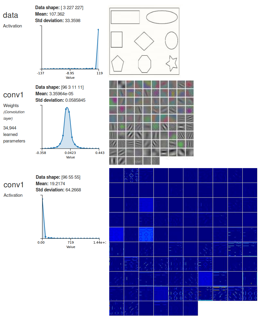
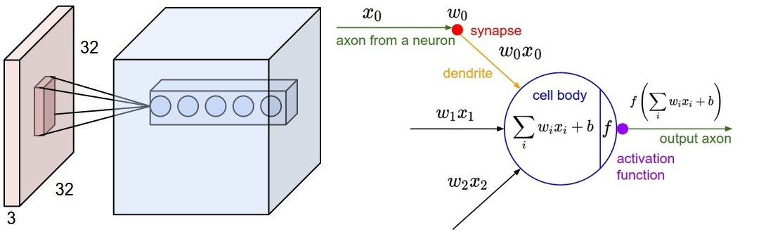
In a CNN it is common practice to split the network into two parts:in the first part, the feature extractor, the data goes through several convolutional layers to extract progressively more complex and abstract features. Convolutional layers are typically interspersed with non-linear transfer functions and pooling layers. Each convolutional layer can be seen as a set of image filters that trigger a high response on a particular pattern. For example, Figure 6 shows a representation of the filters from the first convolutional layer in Alexnet and the activations (the outputs) on a dummy image that contains simple shapes (amusingly, AlexNet classifies the image as a wall clock!). Those filters trigger a high response on shapes like horizontal and vertical edges and corners. For instance, have a look at the filter at the bottom left corner which looks like black-and-white vertical stripes. Now look at the corresponding activations and the high response on vertical lines. Similarly, the next filter immediately at the right shows a high response on oblique lines. Further convolutional layers down the network will be able to trigger a high response on more elaborate shapes like polygons and eventually learn to detect textures and various constituents of natural objects. In a convolutional layer, every output is computed by applying each filter to a window (also known as the receptive field) in the input, sliding the window by the layer stride until the full input has been processed. The receptive field has the same size as the filters. See Figure 7 for an illustration of this behavior. Note that the input window spans across all channels of the input image.
In the second and final part of a CNN, the classifier consists of a number of fully-connected layers, the first of which receives its inputs from the feature extractor. These layers learn complex relationships between features to endow the network with a high-level understanding of the image contents. For example the presence of big eyes and fur might have the network lean towards a cat. How exactly the network makes sense of these features is somewhat magical and another trait of the pure beauty of deep learning. This lack of explainability is sometimes criticized but it is not unlike the way the human brain functions: would you be able to explain how you know that an image of a cat is not an image of a dog?
Fully Convolutional Networks (FCN), as their name implies, consist of only convolutional layers and the occasional non-parametric layers mentioned above. How can eliminating fully-connected layers create a seemingly more powerful model? To answer this question let’s ponder another.
The question is: what is the difference between a fully-connected layer and a convolutional layer? Well that’s simple: in a fully-connected layer, every output neuron computes a weighted sum of the values in the input. In contrast, in a convolutional layer, every filter computes a weighted sum of the values in the receptive field. Wait, isn’t that exactly the same thing? Yes, but only if the input to the layer has the same size as the receptive field. If the input is larger than the receptive field then the convolutional layer slides its input window and computes another weighted sum. This process repeats until the input image has been scanned left to right, top to bottom. In the end, each filter generates a matrix of activations; each such matrix is called a feature map.
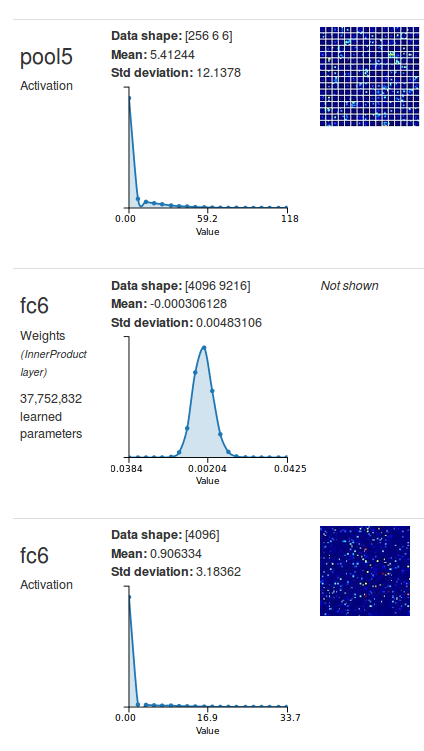
This provides a clue: to replace a fully-connected layer with an equivalent convolutional layer, just set the size of the filters to the size of the input to the layer, and use as many filters as there are neurons in the fully-connected layer. I’ll demonstrate this on the first fully-connected layer in Alexnet (fc6): see Figure 8 for a DIGITS visualization of the layers of interest. You can see that fc6 receives its input from pool5 and the shape of the input is a 256-channel 6×6 image. Besides, the activations at fc6 are a 4096-long vector, which means that fc6 has 4096 output neurons. It follows that if I want to replace fc6 with an equivalent convolutional layer, all I have to do is set the filter size to 6×6 and the number of output feature maps to 4096. As a small digression, how many trainable parameters do you think this layer would have? For every filter there is one bias term plus one weight per number in the receptive field. The receptive field has a depth of 256 and a size of 6×6 therefore there are 256x6x6+1=9217 parameters per filter. Since there are 4096 filters, the total number of parameters for this layer is 37,752,832. That is exactly the number of parameters that DIGITS says fc6 has. All is well so far.
In practice, Replacing the layer is simple. If you are using Caffe, just replace the definition on the left in Table 1 with the definition on the right.
layer {
  name: "fc6"
  type: "InnerProduct"
  bottom: "pool5"
  top: "fc6"
  inner_product_param {
    num_output: 4096

  }
}
|
layer {
  name: "conv6"
  type: "Convolution"
  bottom: "pool5"
  top: "conv6"
  convolution_param {
    num_output: 4096
    kernel_size: 6
  }
}
|
Armed with this knowledge, you can now proceed to converting all the fully-connected layers in Alexnet with their corresponding convolutional layers. Note that you don’t have to use DIGITS to figure out the shapes of the input to those layers; you could calculate them manually. As fun as that may sound, I assure you that you will run out of patience if you need to do this for the 16 layers (plus intervening pooling layers) in VGG-16. Not to mention the fact that you will inevitably lose the scratchpad you used to scribble your notes. Besides, as a Deep Learning fan, you should be comfortable with the idea of letting a machine do the work for you. So let DIGITS do the work for you.
The resulting FCN has exactly the same number of learnable parameters, the same expressivity and the same computational complexity as the base CNN. Given the same input, it will generate the same output. You might wonder: why go through the trouble of converting the model? Well, “convolutionalizing” the base CNN introduces a great amount of flexibility. The model is no longer constrained to operate on a fixed input size (224×224 pixels in Alexnet). It can process larger images by scanning through the input as if sliding a window, and instead of producing a single probability distribution for the whole input, the model generates one per 224×224 window. The output of the network is a tensor with shape KxHxW where K is the number of classes, H is the number of sliding windows along the vertical axis and W is the number of sliding windows along the horizontal axis.
A note on computational efficiency: in theory you could implement the sliding window naively by repeatedly selecting patches of an image and feeding them to a CNN for processing. In practice, this would be computationally very inefficient: as you slide the window incrementally, there is only a small number of new pixels to see at each step. Yet, each patch would need to be fully processed by the CNN, even in the presence of a large overlap between successive patches. You would therefore end up processing each pixel many times. In an FCN, since those computations are all happening within the network, only the minimum number of operations gets to execute so the whole process is orders of magnitude faster.
In summary, that brings us to our first milestone: adding two spatial dimensions to the output of the classification network. In the next section I’ll show you how to further refine the model.
Image Segmentation FCN
The previous section showed how to design an FCN that predicts one class probability distribution per window. Obviously, the number of windows depends on the size of the input image, the size of the window and the step size used between windows when scanning the input image. Ideally, an image segmentation model will generate one probability distribution per pixel in the image. How can you do this in practice? Here again I will employ a method from the FCN paper.
When the input image traverses the successive layers of the “convolutionalized” Alexnet, the pixel data at the input is effectively compressed into a set of coarser, higher-level feature representations. In image segmentation, the aim is to interpolate those coarse features to reconstruct a fine classification, for every pixel in the input. It turns out that this is easily done with deconvolutional layers. These layers perform the inverse operation of their convolutional counterparts: given the output of the convolution, a deconvolutional layer finds the input that would have generated the output, given the definition of the filter. Remember that the stride in a convolutional layer (or a pooling layer) defines how far the window slides when processing the input and is therefore a measure of how down-sampled the output is. Conversely, the stride in a deconvolutional layer is a measure of how up-sampled the output is. Choose a stride of 4 and the output is 4 times bigger!
The next question is: how do I determine how much to up-sample the activations of the final convolutional layer in the model to obtain an output that is the same size as the input image? I need to inspect every layer and carefully write down its scaling factor. Once I have done that for all layers, I just multiply scaling factors together. Let’s look at the first convolutional layer in Alexnet.
layer {
  name: "conv1"
  type: "Convolution"
  bottom: "data_preprocessed"
  top: "conv1"
  convolution_param {
    num_output: 96
    kernel_size: 11
    stride: 4
  }
}
The stride of conv1 is 4, therefore the scaling factor is ¼. Repeating this for all layers, I determine that the total scaling factor in the model is 1/32, as summarised in Table 2. Consequently, the stride I need for the deconvolutional layer is 32.
layer {
  name: "upscore"
  type: "Deconvolution"
  bottom: "score"
  top: "upscore"
  convolution_param {
    num_output: 12 # set this to number of classes
    kernel_size: 63
    stride: 32
  }
}
For the sake of completeness, I have to say that it is not completely true that a convolutional layer with stride \(S\) yields an output that is \(1/S\) times the size of the input in all spatial dimensions. In practice, adding padding \(P > 0\) to the input will increase the number of activations. Conversely, using kernels with size \(K > 1\) will knock activations off the input. At the limit, if you provide the layer with an infinitely long input, the input/output size ratio will indeed be \(1 / S\) in all (spatial) dimensions. In reality, the output of every convolutional (or pooling) layer is shifted by \((P-(K-1)/2)/S\).
For example, consider conv1: since this layer has 100-pixel padding on each side, the output is larger than if there was no padding at all. By applying the above formula we can calculate that each side of the output has, in theory, 23.75 extra pixels. This adds up as we add layers. The cumulative offset across all layers can be computed by walking the graph backwards. The composition of a layer L1 with a layer L2 (i.e. L2 is a bottom of L1 in Caffe terminology), with offsets O1 and O2 respectively, yields an offset of O2/F+O1, where F is the cumulative scaling factor of L2.
See Table 2 for a summary of those computations.
| Layer | Stride | Pad | Kernel size | Scaling Factor (1/S) | Cumulative Scaling Factor |
Offset (P-(K-1)/2)/S |
Cumulative Offset (calculated backward from last layer) |
| conv1 | 4 | 100 | 11 | 1/4 | 1/4 | 23.75 | 18 |
| pool1 | 2 | 0 | 3 | 1/2 | 1/8 | -0.5 | -77 |
| conv2 | 1 | 2 | 5 | 1 | 1/8 | 0 | -73 |
| pool2 | 2 | 0 | 3 | 1/2 | 1/16 | -0.5 | -73 |
| conv3 | 1 | 1 | 3 | 1 | 1/16 | 0 | -65 |
| conv4 | 1 | 1 | 3 | 1 | 1/16 | 0 | -65 |
| conv5 | 1 | 1 | 3 | 1 | 1/16 | 0 | -65 |
| pool5 | 2 | 0 | 3 | 1/2 | 1/32 | -0.5 | -65 |
| conv6 | 1 | 0 | 6 | 1 | 1/32 | -2.5 | -49 |
| conv7 | 1 | 0 | 1 | 1 | 1/32 | 0 | 31 |
| upscore | 32 | 0 | 63 | 32* | 1 | 31* | 31 |
Table 2 shows that the output of the network is shifted by 18 pixels with respect to the input as it traverses all layers from conv1 to upscore. The last trick I need in the segmentation model is a layer to crop the network output and remove the 18 extra pixels on each border. This is easily done in Caffe with a Crop layer, defined in the following listing.
layer {
  name: "score"
  type: "Crop"
  bottom: "upscore"
  bottom: "data"
  top: "score"
  crop_param {
    axis: 2
    offset: 18
  }
}
You might notice that in this version of Alexnet there is a bit more padding than you are used to seeing in that conv1 layer. There are two reasons behind this: one reason is to generate a large initial shift, so the offsets incurred by successive layers do not eat into the image. The main reason, however, is to have the network process the borders of the input image in such a way that they hit the center of the network’s receptive field, approximately.
At last, I now have everything I need to replicate the FCN-Alexnet model from the FCN paper. Let’s relax for a minute and look at some refreshing images from the SYNTHIA dataset.
The SYNTHIA Dataset
The SYNTHIA dataset was originally published in this this paper [5].
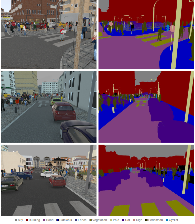
See Figure 9 for sample images from the SYNTHIA dataset. These images show synthetically generated urban scenes with various object classes such as buildings, roads, cars and pedestrians under varying conditions such as day and night. Amusingly, the images look realistic enough that one sometimes feels intrigued by them: hmmm, that man reading a newspaper in the middle of the road on that first picture is acting strangely, he’s certainly up to no good!
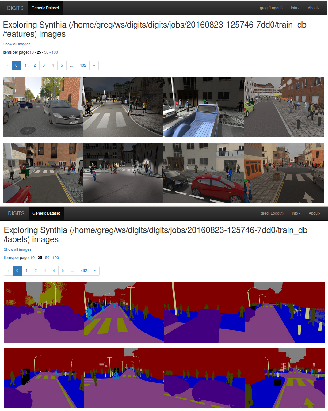
In DIGITS 5.0, creating an image segmentation dataset is as simple as pointing to the input and ground-truth image folders and clicking the “Create” button. DIGITS supports various label formats such as palette images (where pixel values in label images are an index into a color palette) and RGB images (where each color denotes a particular class).
After you have created your dataset in DIGITS you can explore the databases to visually inspect their contents, as in Figure 10.
Training the Model
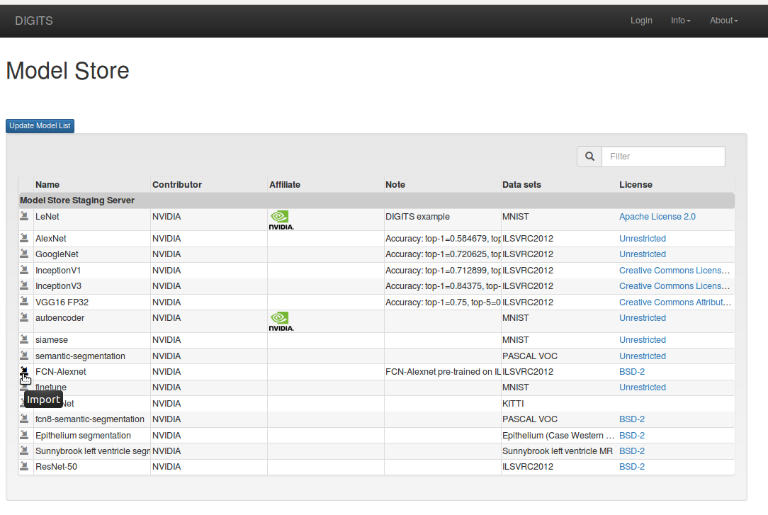
A dataset and a network description are all you need to start training a model in DIGITS. If you thought the process of convolutionalizing Alexnet was somewhat complicated or time consuming then fret not: DIGITS 5.0 comes with a model store and as you can imagine, FCN-Alexnet can be retrieved from the DIGITS model store!
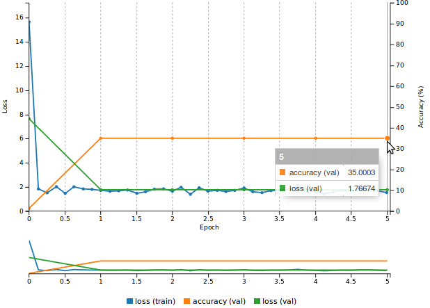
If, however you decided to go the hard way and create the model description yourself, you will want to use a suitable weight initialization scheme like the Kaiming [5] (also known as MSRA) method, which is state of the art in the presence of Rectified Linear Units. This is easily done in Caffe by adding a weight_filler { type: "msra" } directive to your parametric layers. If you train your model this way in DIGITS you will probably end up with a curve that resembles the one in Figure 11. As you can see the performance is less than satisfactory. Validation accuracy plateaus at 35% (meaning that only 35% of pixels in the validation set are correctly labeled). The training loss is in line with the validation loss, indicating that the network is underfitting the training set.
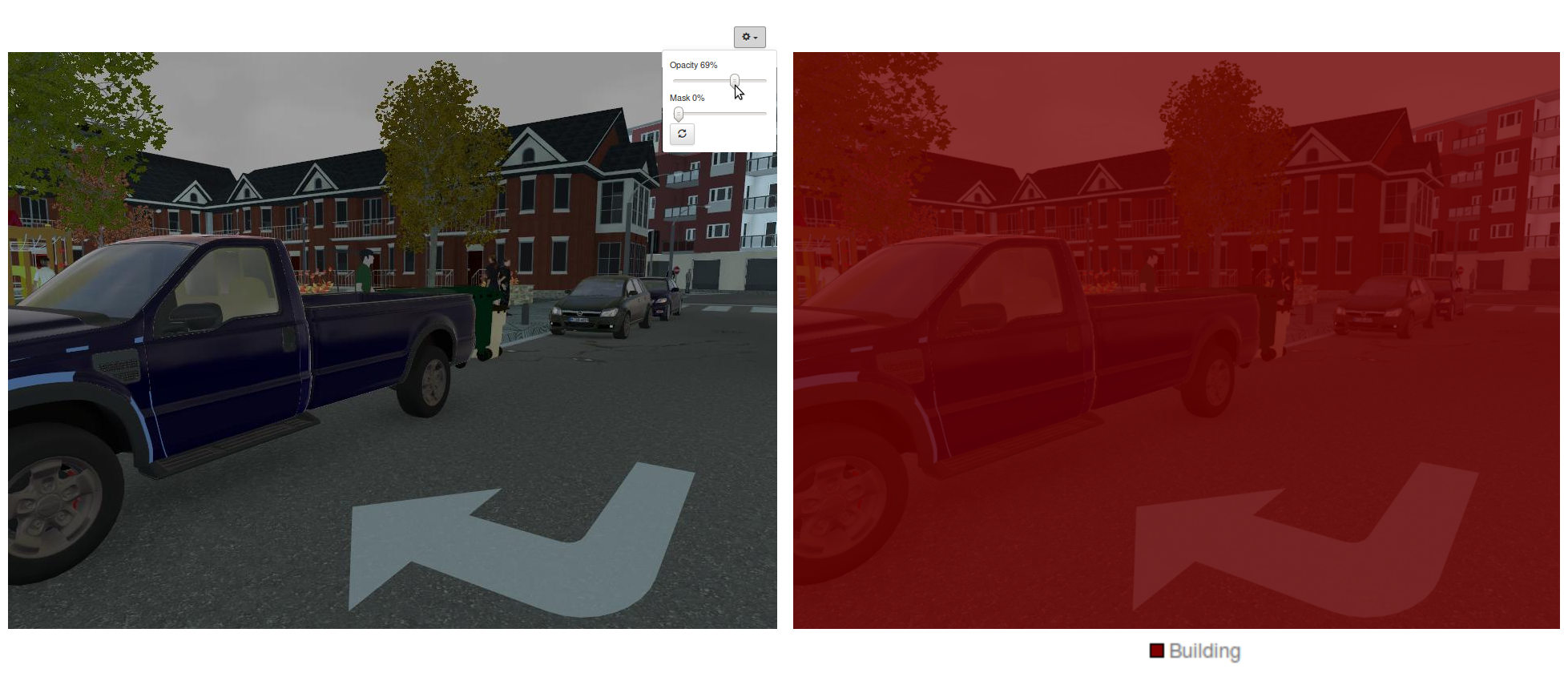
You can try your luck on a sample image and ask DIGITS for a visualization of the image segmentation. You will see something like Figure 12, where you can see that the network is indiscriminately classifying everything as building. It turns out that building is the most represented object class in SYNTHIA and the network has just lazily learnt to achieve 35% accuracy by labeling everything as building. What are commonly accepted ways to deal with a network that underfits the training set?
- Train for longer: looking at the loss curves, this is unlikely to help as training seems to have hit a plateau. The network has entered a local minimum and is unable to get out of it.
- Increase the learning rate, and reduce the batch size: this could encourage a network that is trapped in a local minimum to explore beyond its immediate surroundings, although this increases the risk that the network diverges.
- Increase the size of the model: this could increase the expressivity of the model.
Another method that I found to work extremely well in computer vision is transfer learning. Read on to find out more!
Transfer Learning
You don’t have to start from randomly initialized weights to train a model. In a lot of cases, it helps to reuse knowledge that a network learned when training on another dataset. This is particularly true in Computer Vision through CNNs since a lot of low-level features (lines, corners, shapes, textures) immediately apply to any dataset. Since image segmentation does classification at the pixel level it makes sense to transfer learning from image classification datasets such as ILSVRC2012. This turns out to be rather straightforward when using Caffe—with one or two gotchas of course! Remember that in Alexnet’s fc6, the weights have a shape of 4096×9216. In FCN-Alexnet’s conv6, the weights have a shape of 4096x256x6x6. This is exactly the same number of weights, but since the shapes are different, Caffe will be unable to automatically carry the weights over to FCN-Alexnet. This operation may be performed using a net surgery script, an example of which can be found in the DIGITS repository on Github. The function of the net surgery script is to transplant parameters from fully-connected layers to their convolutional counterparts. You may however find it easier to simply download the pretrained model from the public DIGITS Model Store! Figure 13 shows a preview of the model store: click “Import” next to “FCN-Alexnet” and DIGITS will download the pre-trained model.
Another related concern that you might have is how to initialize the upsampling layer added earlier in this post, since this layer isn’t part of the original Alexnet model: in the FCN paper the recommendation is to randomly initialize the corresponding weights and have the network learn them. The authors of the paper later realized that it is just as simple to initialize these weights in such a way that the layer just acts as a magnifying glass, by doing bilinear interpolation. In Caffe this is done by adding a weight_filler {type: "bilinear"} directive to the layer.
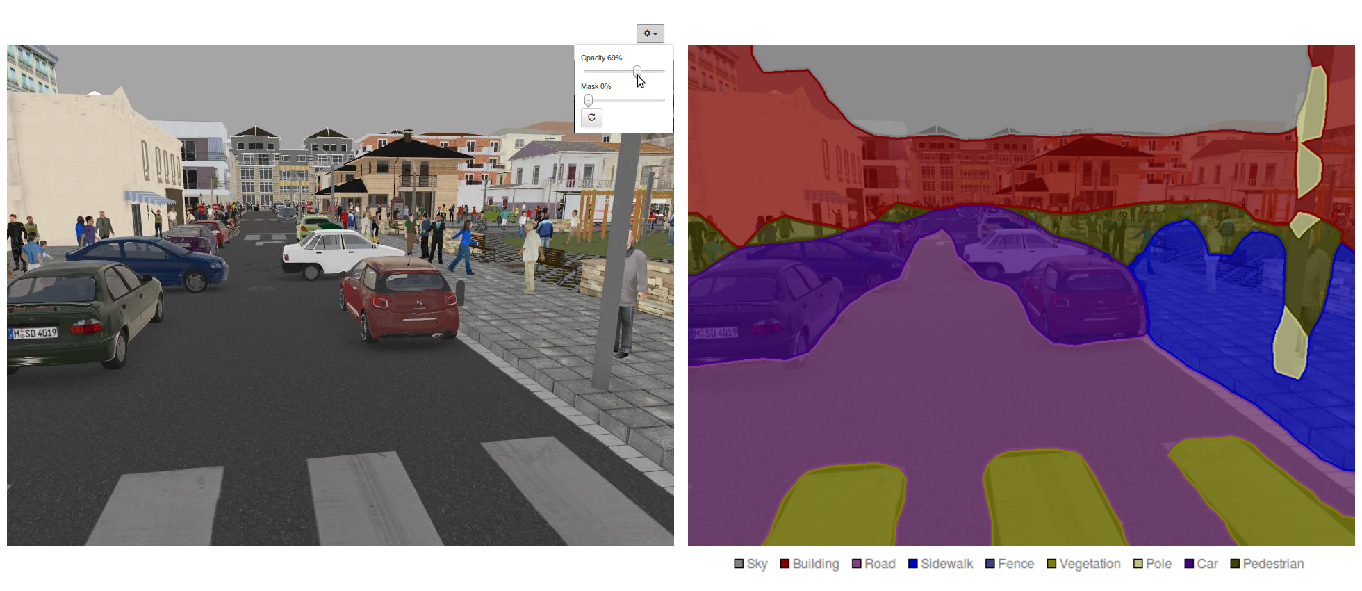
Using a pre-trained FCN-Alexnet model, you will notice that the accuracy quickly exceeds 90% and when testing individual images such as in Figure 14 the result will be a much more convincing image segmentation, with detections for 9 different object classes. You might, however, be slightly disappointed to see that object contours are very coarse. Read on to the next and final section to discover how to further improve the precision and accuracy of our segmentation model.
Enabling Finer Segmentation
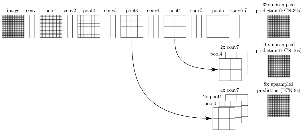
Remember that the new upsampling layer added to FCN-Alexnet magnifies the output of conv7 by a factor of 32. In practice, this means that the network makes a single prediction per 32×32 pixel block, which explains why object contours are so coarse. The FCN paper introduces another great idea for addressing this limitation: skip connections are added to directly redirect the output of pool3 and pool4 towards the output of the network. Since those pooling layers are further back in the network, they operate on lower-level features and are able to capture finer details. In a network architecture called FCN-8s the FCN paper introduces a VGG-16-based network in which the final output is an 8x upsampling of the sum of pool3, a 2x upsampling of pool4 and a 4x upsampling of conv7, as Figure 15 illustrates. This leads to a network that is able to make predictions at a much finer grain, down to 8×8 pixel blocks.
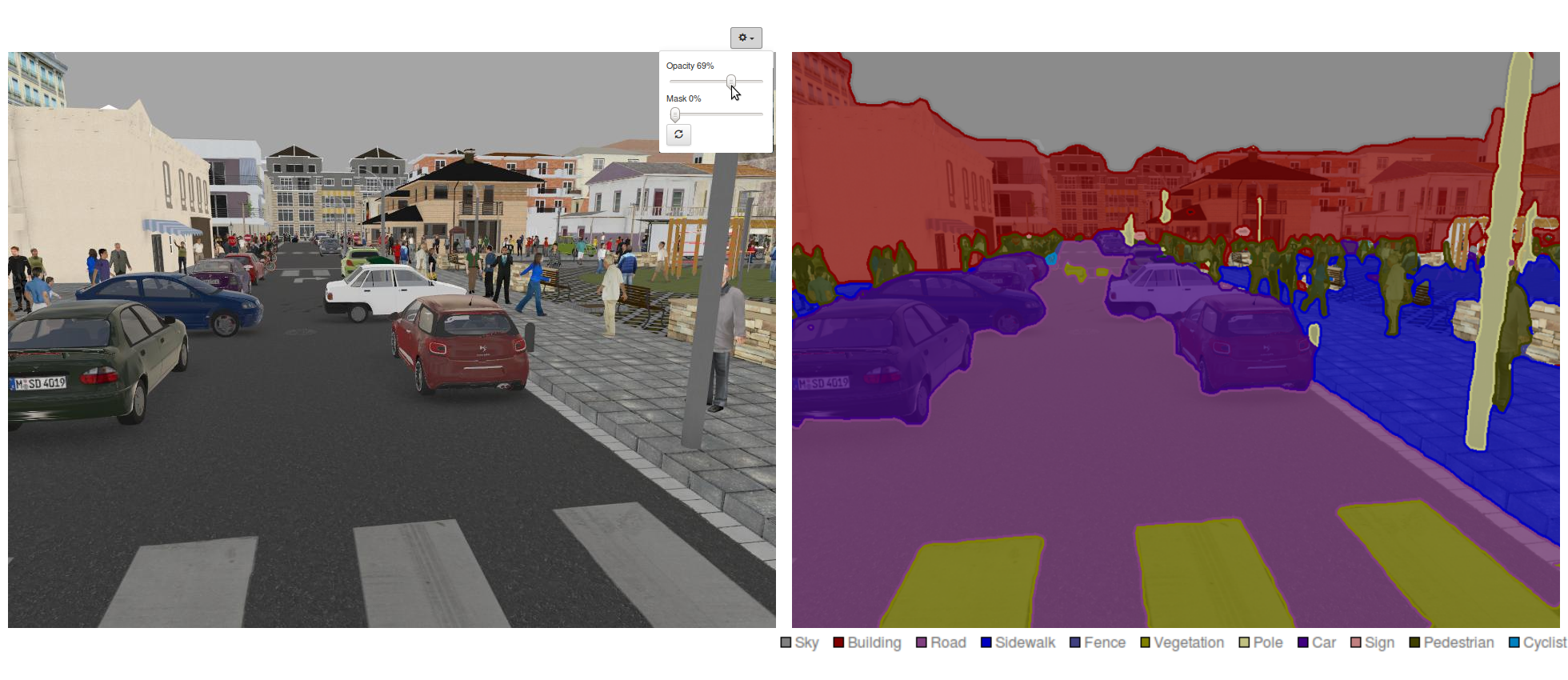
For your convenience, a pre-trained FCN-8s can be downloaded from the public DIGITS model store. (You don’t want to manually convolutionalize VGG-16!) If you train FCN-8s on SYNTHIA using DIGITS, you should see that the validation accuracy exceeds 95% after only a couple of epochs. Most importantly, when you test a sample image and observe DIGITS’ superb image segmentation visualization, you will see much sharper object contours, as in Figure 16.
Now It’s Your Turn!
After reading this post, you should have the information you need to get started with image segmentation. The DIGITS 5 general release will be available in the first week of December. Visit the DIGITS page to learn more and sign up for the NVIDIA Developer program to be notified when it is ready for download.
DIGITS is an open-source project on GitHub. If you’d like to start experimenting with image segmentation right away, head over to the DIGITS GitHub project page where you can get the source code. We look forward to your feedback and contributions on Github as we continue to develop it.
Please let us know how you are doing by commenting on this post!
Acknowledgements
I would like to thank Mark Harris for his insightful comments and suggestions.
References
[1] Krizhevsky, A., Sutskever, I. and Hinton, G. E. “ImageNet Classification with Deep Convolutional Neural Networks”. NIPS Proceedings. NIPS 2012: Neural Information Processing Systems, Lake Tahoe, Nevada. 2012.
[2] Christian Szegedy, Wei Liu, Yangqing Jia, Pierre Sermanet, Scott Reed, Dragomir Anguelov, Dumitru Erhan, Vincent Vanhoucke, Andrew Rabinovich. “Going Deeper With Convolutions”. CVPR 2015.
[3] Simonyan, Karen, and Andrew Zisserman. “Very deep convolutional networks for large-scale image recognition.” arXiv technical report arXiv:1409.1556. 2014.
[4] Long, Jonathan, Evan Shelhamer, and Trevor Darrell. “Fully convolutional networks for semantic segmentation.” Proceedings of the IEEE Conference on Computer Vision and Pattern Recognition 2015: 3431-3440.
[5] Ros, German, Laura Sellart, Joanna Materzynska, David Vazquez, and Antonio M. Lopez; “The SYNTHIA Dataset: A large collection of synthetic images for semantic segmentation of urban scenes.” Proceedings of the IEEE Conference on Computer Vision and Pattern Recognition 2016: 3234-3243.
[6] He, Kaiming, Xiangyu Zhang, Shaoqing Ren, and Jian Sun “Delving deep into rectifiers: Surpassing human-level performance on imagenet classification.” Proceedings of the IEEE International Conference on Computer Vision 2015: 1026-1034.