
Data scientists across various domains use clustering methods to find naturally ‘similar’ groups of observations in their datasets. Popular clustering methods can be:
- Centroid-based: grouping points into k sets based on closeness to some centroid.
- Graph-based: grouping vertices in a graph based on their connections.
- Density-based: more flexibly grouping based on density or sparseness of data in a nearby region.
The Hierarchical Density-Based Spatial Clustering of Applications w/ Noise (HDBSCAN) algorithm is a density-based clustering method that is robust to noise (accounting for points in sparser regions as either cluster boundaries and directly labeling some of them as noise). Density-based clustering methods, like HDBSCAN, are able to find oddly-shaped clusters of varying sizes — quite different from centroid-based clustering methods like k-means, k-medioids, or gaussian mixture models, which find a set of k centroids to model clusters as balls of a fixed shape and size. Aside from having to specify k in advance, the performance and simplicity of centroid-based algorithms have helped them remain among the most popular methods for clustering points in high dimensions; even though they can’t model clusters of varying size, shape, or density without modifications to the input data points.
HDBSCAN builds upon a well-known density-based clustering algorithm called DBSCAN, which doesn’t require the number of clusters to be known ahead of time but still has the unfortunate shortcoming that assumes clusters can be modeled with a single global density threshold. This makes it difficult to model clusters with varying densities. HDBSCAN improves upon this shortcoming by using single-linkage agglomerative clustering to build a dendrogram, which allows it to find clusters of varying densities. Another well-known density-based clustering method that improves upon DBSCAN and uses hierarchical clustering to find clusters of varying densities is called the OPTICS algorithm. OPTICS improves upon the standard single-linkage clustering by projecting the points into a new space, called reachability space, which moves the noise further away from dense regions, making it easier to handle. However, like many other hierarchical agglomerative clustering methods, such as single- and complete-linkage clustering, OPTICS comes with the shortcoming of cutting the resulting dendrogram at a single global cut value. HDBSCAN is essentially OPTICS+DBSCAN, introducing a measure of cluster stability to cut the dendrogram at varying levels.
We’re going to demonstrate the features currently supported in the RAPIDS cuML implementation of HDBSCAN with quick examples and will provide some real-world examples and benchmarks of our implementation on the GPU. After reading this blog post, we hope you’re excited about the benefits that the RAPIDS’ GPU-accelerated HDBSCAN implementation can provide to your workflows and exploratory data analysis process.
Getting started with HDBSCAN in RAPIDS
RAPIDS provides a set of GPU-accelerated Python libraries that are near drop-in replacements for many popular libraries in the PyData ecosystem. The example notebook below demonstrates the API compatibility between the most widely-used HDBSCAN Python library on the CPU and RAPIDS cuML HDBSCAN on the GPU (spoiler alert – in many cases, it’s as easy as changing an import).
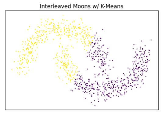
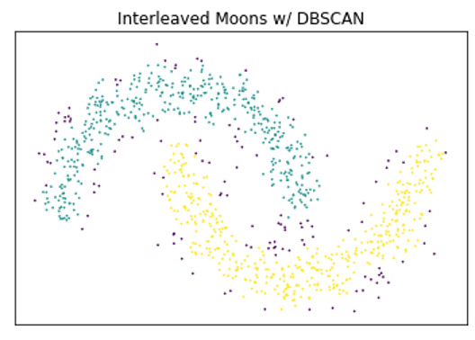
Below is a very simple example demonstrating the benefits of density-based clustering over centroid-based techniques on certain types of data, as well as the benefits of using HDBSCAN over DBSCAN.
A very basic comparison of the benefits of density-based clustering compared to different clustering algorithms.
HDBSCAN in Practice
Density-based clustering techniques are a natural fit for many different clustering tasks since they are able to find oddly shaped clusters of varying sizes. Like many other general-purpose machine learning algorithms, there’s no free lunch, so while HDBSCAN has improved on some well-established algorithms, it is still not always going to be the best tool for the job. That said, DBSCAN and HDBSCAN have found notable success in applications ranging from geospatial and collaborative filtering / recommender systems to finance and scientific computing, being used in disciplines ranging from astronomy to accelerator physics to genomics. It’s robustness to noise also makes it useful for outlier and anomaly detection applications.
As with so many other tools in the data analysis and machine learning ecosystem, computation time has a large impact on production systems and iterative workflows. A faster HDBSCAN means being able to try out more ideas and make better models. Below are a couple of example notebooks that use HDBSCAN to cluster word embeddings and single-cell RNA gene expressions. These are meant to be brief and provide a nice starting point for using HDBSCAN with your own datasets. Have you successfully applied HDBSCAN in industry or in a scientific discipline which we’ve not listed here? Please leave a comment because we would love to hear about it. If you run the example notebooks on your own hardware, please also let us know about your setup and your experience with RAPIDS.
Word Embeddings
Vector embeddings represent a popular and very broad range of machine learning applications for clustering. We’ve chosen the GoogleNews dataset because it’s large enough to provide a good indication of our algorithm’s scale and yet small enough that it can be executed on a single machine. The following notebook demonstrates the use of HDBSCAN to find meaningful topics, which arise from highly dense regions in the angular space of word embeddings and uses UMAP to visualize the resulting topic clusters. It uses a subset of the entire dataset for visualization purposes but provides a great demo for tweaking the different hyperparameters and getting familiar with their effect on the resulting clusters. We benchmarked the entire dataset with the default hyperparameter settings, which has a shape of 3Mx300, and stopped the Scikit-learn contrib implementation on the CPU after 24 hours. The RAPIDS implementation took roughly ~22.8mins.
Single-Cell RNA
Below is an example workflow based on tutorial notebooks from the Scanpy and Seurat libraries. This example notebook is taken from the RAPIDS single-cell examples repository, which also contains several notebooks demonstrating the use of RAPIDS for single-cell and tertiary analysis. On a DGX-1 (Intel 40-core Xeon CPU + NVIDIA V100 GPU), we found a 29x speedup for HDBSCAN (~1s on the GPU instead of ~29s with multiple CPU threads) using the first 50 principal components on a dataset containing the gene expressions for ~70k lung cells.
Accelerating HDBSCAN on GPUs

The RAPIDS cuML project includes an end-to-end, GPU-accelerated HDBSCAN and provides both Python and C++ APIs. As with many of the neighborhood-based algorithms in cuML, it leverages the brute-force kNN from Facebook’s FAISS library to accelerate the construction of the kNN graph in mutual reachability space. This is currently a major bottleneck, and we’re working on ways to improve it further with options for both exact and approximate nearest neighbors.
cuML also includes an implementation of single-linkage hierarchical clustering, which provides both C++ and Python APIs. GPU-acceleration of the single-linkage algorithm required a new primitive to compute the minimum spanning tree. This primitive is graph-based so that it can be reused across both the cugraph and cuml libraries. Our implementation allows restarting so that we can connect an otherwise disconnected knn graph and improve scalability by not having to store an entire matrix of pairwise distances in GPU memory.
As with most of the C++ algorithms in cuML, these rely heavily on the RAPIDS Analytics Framework Toolkit project (RAFT) for most of our ML and Graph-based primitives. Finally, they leverage the great work done by Leland McInnes and John Healy to GPU-accelerate even the cluster condensing and selection steps, keeping the data on the GPU as much as possible and providing an additional boost to performance as data sizes scale into the millions.
Benchmarks
We used a benchmark notebook provided by the reference implementation on CPU from McInnes et al. to compare it against cuML’s new GPU implementation. The reference implementation is highly optimized for cases of lower dimensionality, and we compare the higher dimensional cases against the brute-force implementation, which makes heavy use of Facebook’s FAISS library.
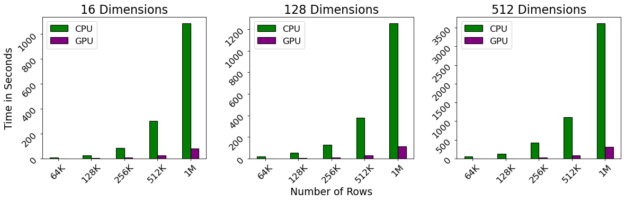
Benchmarks were performed on a DGX-1, which contains a 40-core Intel Xeon CPU and NVIDIA 32gb V100 GPUs. Even with a linear scaling with respect to the number of dimensions and quadratic scaling with respect to the number of rows, we observe that the GPU still maintains near-interactive performance even as the number of rows exceeds 1M.

What’s in Flux?
While we have successfully implemented the core of the HDBSCAN algorithm on the GPU, opportunities remain to improve its performance even further, such as by speeding up the brute-force kNN graph construction, pruning out distance computations, and even using an approximate kNN. While Euclidean distance covers the widest range of uses, we would also like to expose other distance metrics which are available in the Scikit-learn Contrib implementation.
The scikit-learn contrib implementation also contains a lot of nice additional features which are not included in the seminal paper on HDBSCAN, such as semi-supervised and fuzzy clustering. We also have the building blocks for robust single-linkage and the OPTICS algorithm, which would be nice future additions to RAPIDS. Finally, we’re hoping to support sparse inputs in the future.
If you find that one or more of these features could make your application or data analysis project more successful, even if it’s not listed here, head on over to our Github project and create an issue.
Summary
HDBSCAN is a relatively new density-based clustering algorithm that “stands on the shoulders of giants”, improving upon the well-known DBSCAN & OPTICS algorithms. In fact, it’s core primitives have also increased reuse and provided building-blocks for other algorithms, such as a graph-based minimum spanning tree and single-linkage clustering within the RAPIDS ML and Graph libraries.
Like other algorithms for data modeling, HDBSCAN is not the perfect tool for every job, however it has found much practical use in both industry and scientific computing applications. It can also be a great companion alongside dimensionality reduction algorithms like PCA or UMAP, especially when used in exploratory data analysis applications.
