
HDBSCAN is a state-of-the-art, density-based clustering algorithm that has become popular in domains as varied as topic modeling, genomics, and geospatial analytics.
RAPIDS cuML has provided accelerated HDBSCAN since the 21.10 release in October 2021, as detailed in GPU-Accelerated Hierarchical DBSCAN with RAPIDS cuML – Let’s Get Back To The Future. However, support for soft clustering (also known as fuzzy clustering) was not included. With soft clustering, a vector of values (rather than a single cluster label) is created for each point representing the probability that the point is a member of each cluster.
Performing HDBSCAN soft clustering on CPUs has been slow. It can take hours or even days on medium-sized datasets due to the heavy computational burden. Now, in the 22.10 RAPIDS release, cuML provides accelerated soft clustering for HDBSCAN, enabling the use of this technique on large datasets.
This post highlights the importance of using soft clustering to better capture nuance in downstream analysis and the performance gains possible with RAPIDS. In a document clustering example, soft clustering that takes hours on a CPU can be completed in seconds with cuML on a GPU.
Soft clustering code
In the CPU-based scikit-learn-contrib/hdbscan library, soft clustering is available through the all_points_membership_vectors top-level module function.
cuML matches this API:
import cuml

blobs, labels = cuml.datasets.make_blobs(n_samples=2000, n_features=10, random_state=12)

clusterer = cuml.cluster.hdbscan.HDBSCAN(prediction_data=True)
clusterer.fit(blobs)
cuml.cluster.hdbscan.all_points_membership_vectors(clusterer)
Why soft clustering
In many clustering algorithms, each record in a dataset is either assigned to a single cluster or considered noise and not assigned to any clusters. However, in the real world, many records do not perfectly fit into a single cluster. HDBSCAN acknowledges this reality by providing a mechanism for soft clustering by representing the degree to which each point belongs to each cluster. This is similar to other algorithms such as mixture models and fuzzy c-means.
Imagine a news article about a sports-themed musical. If you wanted to assign the article to a cluster, would it belong to a sports cluster or a musical cluster? Perhaps a smaller cluster specifically for sports-themed musicals? Or should it have some level of membership in both clusters?
By forcing the choice of a single label, this nuance is lost, which can be significant when the results of clustering are used for downstream analysis or actions. If only a sports label is assigned, would a recommendation system surface the article to readers also interested in musicals? What about the inverse (a reader interested in one but not the other)? This article should be potentially in the queue for readers interested in either or both of these topics.
Soft clustering solves this problem, enabling actions based on thresholds for each category and creating applications that provide a better experience.
Example of document clustering
You can use document clustering to measure the potential real-world performance benefits and impact of cuML’s accelerated soft clustering.
Many modern document clustering workflows are composed of the following steps:
- Convert each document into a numeric representation (often using neural network embeddings)
- Reduce the dimensionality of the numeric-transformed documents
- Perform clustering on the dimension-reduced dataset
- Take actions based on the results
If you would like to run the workflow on your system, a Jupyter Notebook is available by visiting hdbscan-blog.ipynb on GitHub.
Preparing the dataset
This example uses the A Million News Headlines dataset from Kaggle, which contains over 1 million news article headlines from the Australian Broadcasting Corporation.
After downloading the dataset, convert each headline into an embedding vector. To do this, use the all-MiniLM-L6-v2 neural network from the Sentence Transformers library. Note that a few other libraries imported will be used later.
import numpy as np
import pandas as pd
import cuml
from sentence_transformers import SentenceTransformer

N_HEADLINES = 10000

model = SentenceTransformer('all-MiniLM-L6-v2')

df = pd.read_csv("/path/to/million-headlines.zip")
embeddings = model.encode(df.headline_text[:N_HEADLINES])
Reducing dimensionality
With the embeddings ready, reduce the dimensionality down to five features using cuML’s UMAP. This example is only using 10,000 records, as it is intended as a guide.
For reproducibility, set a random_state. The results in this workflow may differ slightly when run on your machine, depending on the UMAP results.
umap = cuml.manifold.UMAP(n_components=5, n_neighbors=15, min_dist=0.0, random_state=12)
reduced_data = umap.fit_transform(embeddings)
Soft clustering
Next, fit the HDBSCAN model on the dataset and enable using all_points_membership_vectors for soft clustering by setting prediction_data=True. Also set min_cluster_size=50, which means that groupings of fewer than 50 headlines will be considered as part of another cluster (or noise), rather than as a separate cluster.
clusterer = cuml.cluster.hdbscan.HDBSCAN(min_cluster_size=50, metric='euclidean', prediction_data=True)
clusterer.fit(reduced_data)
soft_clusters = cuml.cluster.hdbscan.all_points_membership_vectors(clusterer)
soft_clusters[0]
array([0.01466704, 0.01035215, 0.0220814 , 0.01829496, 0.0127591 ,
       0.02333117, 0.01993877, 0.02453639, 0.03369896, 0.02514531,
       0.05555269, 0.04149485, 0.05131698, 0.02297594, 0.03559102,
       0.02765776, 0.04131499, 0.06404213, 0.01866449, 0.01557038,
       0.01696391], dtype=float32)
Inspecting a couple of clusters
Before going further, look at the assigned labels (-1 represents noise). It is evident that there are quite a few clusters in this data:
pd.Series(clusterer.labels_).value_counts()
-1     3943
 3     1988
 5     1022
 20     682
 13     367
 7      210
 0      199
 2      192
 8      190
 16     177
 12     161
 17     143
 15     107
 19      86
 9       83
 11      70
 4       68
 18      66
 6       65
 10      61
 1       61
 14      59
dtype: int64
Select two clusters at random, clusters 7 and 10, for example, and examine a few points from each.
df[:N_HEADLINES].loc[clusterer.labels_ == 7].headline_text.head()
572    man accused of selling bali bomb chemicals goe...
671      timor sea treaty will be ratfied shortly martin
678     us asks indonesia to improve human rights record
797           shop owner on trial accused over bali bomb
874    gatecrashers blamed for violence at bali thank...
Name: headline_text, dtype: object

df[:N_HEADLINES].loc[clusterer.labels_ == 10].headline_text.head()
40     direct anger at govt not soldiers crean urges
94                   mayor warns landfill protesters
334                    more anti war rallies planned
362     pm criticism of protesters disgraceful crean
363      pm defends criticism of anti war protesters
Name: headline_text, dtype: object
Then, use the soft clustering membership scores to find some points, which might belong to both of the clusters. From the soft cluster scores, identify the top two clusters for each point. Exclude outliers by filtering for soft memberships to clusters 7 and 10, which are both proportionately larger than their memberships to other clusters:
df2 = pd.DataFrame(soft_clusters.argsort()[:,::-1][:,:2])
df2["sum"] = soft_clusters.sum(axis=1)
df2["cluster_7_ratio"] = soft_clusters[:,7] / df2["sum"]
df2["cluster_10_ratio"] = soft_clusters[:,10] / df2["sum"]
df2[(df2[0] == 7) & (df2[1] == 10) & (df2["cluster_7_ratio"] > 0.1) & (df2["cluster_10_ratio"] > 0.1)]

3824  7  10  0.630313         0.170000         0.160453
6405  7  10  0.695286         0.260162         0.119036
Inspect the headlines for these points, and notice they are both about Indonesia, which is also in the cluster 7 headline 678 (above). Also notice that both of these headlines are about antiwar and peace, which are topics included in several of the cluster 10 headlines.
df[:N_HEADLINES].iloc[3824]
publish_date                                              20030309
headline_text    indonesians stage mass prayer against war in iraq
Name: 3824, dtype: object

df[:N_HEADLINES].iloc[6405]
publish_date                           20030322
headline_text    anti war fury sweeps indonesia
Name: 6405, dtype: object
Why soft clustering matters
How confident should you be that these results belong to their assigned cluster, rather than another cluster? As previously observed, some clusters contain headlines that have a meaningful probability of being in a different cluster.
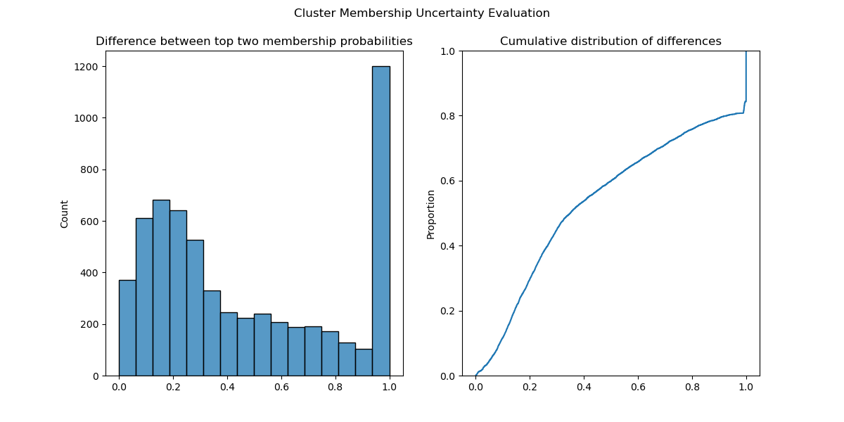
The degree of confidence can be partially quantified by calculating the difference between the membership probabilities of each point’s top two clusters, as noted in the HDBSCAN documentation. This example excludes noise points, to drive home how this does not just happen with “noisy” points, but also those assigned cluster labels:
soft_non_noise = soft_clusters[clusterer.labels_ != -1]
probs_top2_non_noise = np.take_along_axis(soft_non_noise, soft_non_noise.argsort(), axis=1)[:, -2:]
diffs = np.diff(probs_top2_non_noise).ravel()
Plotting a histogram and the empirical cumulative distribution function of these differences shows that many points were close to being assigned a different cluster label. In fact, about 30% of points had top-two cluster membership probabilities within 0.2 of one another (Figure 1).
Using these soft clustering probabilities enables you to incorporate this uncertainty to build much more robust machine learning pipelines and applications.
Performance benchmark results
Next, run the preceding core workload on different numbers of news article headlines, varying from 25,000 to 400,000 rows. Note that HDBSCAN parameters can be tweaked for larger datasets.
For this example, CPU benchmarks were run on an x86 Intel Xeon Gold 6128 CPU at 3.40 GHz. GPU benchmarks were recorded on an NVIDIA Quadro RTX 8000 with 48 GB of memory.
On the CPU (indicated by the hdbscan backend), soft clustering performance scales loosely linearly as the number of documents is doubled. 50,000 documents took 50 seconds; 100,000 documents took 500 seconds; 200,000 documents took 5,500 seconds (1.5 hours); and 400,000 documents took over 60,000 seconds (17 hours). See Table 1 for more details.
Using the GPU-accelerated soft clustering in cuML, soft clusters for 400,000 documents can be calculated in less than 2 seconds, rather than 17 hours.
| Backend | Number of Rows | Soft Clustering Time (s) |
| cuml | 25,000 | 0.008182 |
| hdbscan | 25,000 | 5.795254 |
| cuml | 50,000 | 0.014839 |
| hdbscan | 50,000 | 53.847145 |
| cuml | 100,000 | 0.077507 |
| hdbscan | 100,000 | 485.847746 |
| cuml | 200,000 | 0.322825 |
| hdbscan | 200,000 | 5503.697239 |
| cuml | 400,000 | 1.343359 |
| hdbscan | 400,000 | 62428.348942 |
all_points_membership_vectors with the cuML and CPU backendsIf you would like to run this benchmark on your system, use the benchmark-membership-vectors.py GitHub gist. Note that performance will vary depending on the CPU and GPU used.
Key takeaways
We are excited to report these performance results. Soft clustering can meaningfully improve workflows powered by machine learning. Until now, using a clustering technique like HDBSCAN has been computationally challenging for even a few hundred thousand records.
With the addition of HDBSCAN soft clustering, RAPIDS and cuML continue to break through barriers and make state-of-the-art computational techniques more accessible at scale.
To get started with cuML, visit the RAPIDS Getting Started page, where conda packages, pip packages, and Docker containers are available. cuML is also available in the NVIDIA optimized PyTorch and Tensorflow Docker containers on NVIDIA NGC, making this end-to-end workflow even easier.
Acknowledgments
This post describes cuML functionality contributed by Tarang Jain during his internship at NVIDIA under the mentorship of Corey Nolet.
