
Quantitative developers need to run back-testing simulations to see how financial algorithms perform from a profit and loss (P&L) standpoint. Statistical techniques are important to visualize the possible outcomes of the algorithms in terms of the possible P&L paths. GPUs can greatly reduce the amount of time needed to do this.
In the broader picture, mathematical modeling of financial markets is a practice that goes back to the Nobel Prize-winning Black-Scholes model of 1973. It was revolutionary at the time and has impacted capital markets ever since. The approach of statistical Monte Carlo simulations to represent the price paths achievable with Brownian motion models involve custom models that are tailored to how the markets behave when examining the market microstructure.
This post presents a hardware acceleration study that applies to market participants in the financial markets. The market participants can be:
- Traders, responsible for profitable strategies
- Exchanges, providing the ability for firms to buy and sell securities
- Risk managers, who ensure that a firm’s set of positions are not risking too much of a firm’s capital
These market participants all collaborate on the world’s exchanges where there is a very specific set of rules about prices, volumes, and timing known as the dynamic order book for trading securities.
GPUs provide the accelerated computing needed for simulating these dynamic order books due to the huge amount of pricing data and the speed of execution. This post explains how to apply GPUs in this setting.
Nanosecond-timestamped market transactions are of interest to market participants today, and especially to those in the high-frequency trading space expecting to gain positive profit through accurate predictions. In this context, alpha is a measure of the excess return of an investment relative to the market index, accounting for the risk-free rate and adjusted for risk.
Following the algorithmic and high-frequency trading simulation approach of the book Algorithmic and High-Frequency Trading, and using code samples from Market Making at the Touch with Short-Term Alpha, it’s possible to select a set of stochastic processes and gain timeliness for users, as reported in the timing chart. Buy Low, Sell High: A High Frequency Trading Perspective is a quite-readable alternative on the overall problems solved in these high-frequency markets from a quantitative perspective.
During the study we found that the longer the range of simulated time, the more hardware acceleration provided. The market practitioner will decide the range needed to gain confidence in the simulations as preparation for deploying these simulation techniques in live trading. NVIDIA Hopper and NVIDIA Blackwell architectures both provide over 14,000 internal CUDA cores to provide massively parallel program execution, no matter which NVIDIA GPU model is used: H100 NVL, H100 SXM, H200 NVL, H200 SXM, GH200, B200, or GB200.
The order book and the problem to solve
The amount of market data captured in the world-wide financial markets on a high-frequency basis is staggering. The actual order book and, hence, simulations of the order book, consist of a complex state that includes:
- Price levels at which counterparty bids to buy are placed
- Price levels at which counterparty offers to sell, or asks, are placed
- Midprice, which is the average of the highest bid and the lowest ask
There are 10 levels of bid and 10 levels of ask. Limits orders (LO) are typically placed by counterparties who are specific about price points. Market orders (MO) are placed by counterparties that are more flexible on the execution price but need the trade executed immediately. Researchers and practitioners focus on models to capture profit as these dynamic events occur by placing LOs and MOs in sequence on the exchange of choice. Simulating the strategies is important because of the amount of capital allocated to them by firms.
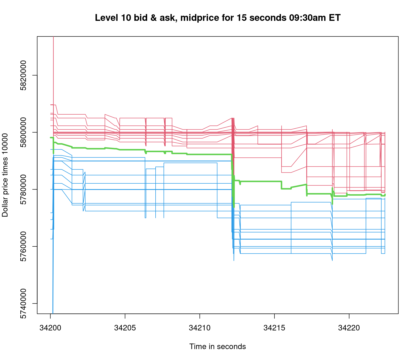
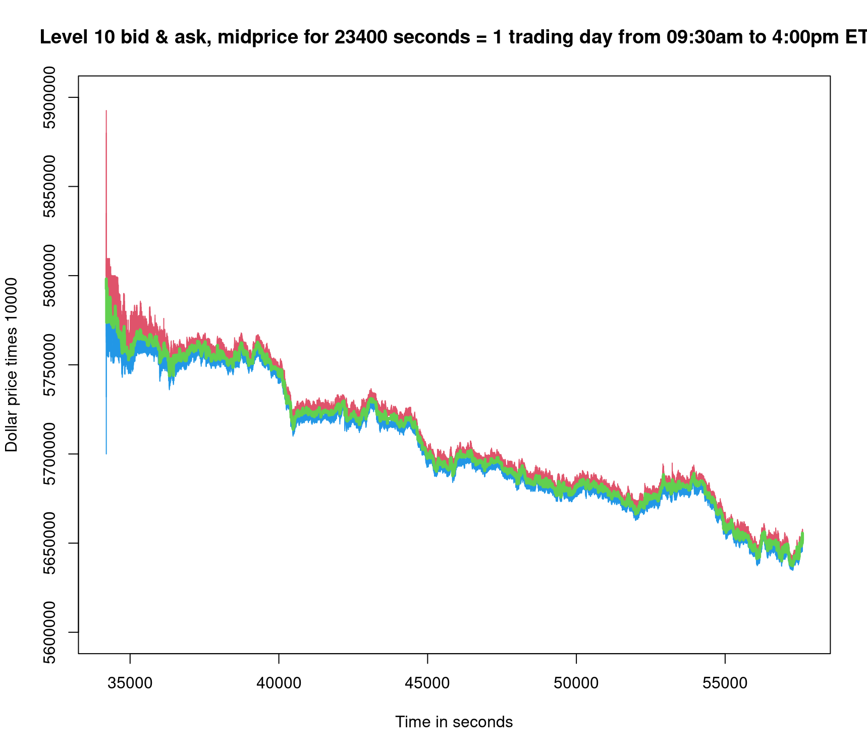
Figures 1 and 2 provide a perspective view for 15 seconds and 23,400 seconds (or one trading day), respectively, of the order book. In Figure 1, the limit order book for a given stock jumps down in the middle of the 15-second view. As a result, the midprice lowers by about $1 from about $579.00 per share to about $578.00 per share. The initial time stamp of 34,200 represents the 9:30 a.m. ET market opening. Note at 34,212 seconds the extreme swing in price at the market open.
This example is a large-cap tech stock. The trading range is wider for the entire day, as there is more time for the market price to be impacted by all the LO and MO activity. In Figure 2 the midprice travels down $14 from about $579.00 per share to about $565.00 per share. The width of the limit order book from top to bottom narrows as time moves away from the market open of the trading day.
Statistical Monte Carlo simulations need to be accelerated with GPUs because they are a good fit to the problem and make the researchers more efficient with their time. A specific implementation of the approach used is sampled for one of the main market simulation modules.
Accelerating simulations with CUDA Python: CuPy versus Numba
Python does not require statements to be contained inside a function, so you can think of Python programs as statements alternating inside and outside a series of functions. Generally speaking, the CuPy approach works well for GPU execution when writing code outside of functions. It is convenient to use CuPy in place of NumPy. An example of the use of CuPy is shown below.
import cupy as cp
x = cp.array([1, 2, 3, 4, 5])
y = cp.array([5, 4, 3, 2, 1])
z = x * y # GPU-accelerated operation
The following is the equivalent code illustrated using Numba:
import numba
from numba import cuda
@cuda.jit
def mult_kernel(x, y, z):
    i = cuda.grid(1)
    if i < x.size:
        z[i] = x[i] * y[i]

# Example usage of Python Numba kernel:
import numpy as np
x = np.array([1, 2, 3, 4, 5], dtype=np.float32)
y = np.array([5, 4, 3, 2, 1], dtype=np.float32)
z = np.zeros_like(x)
mullt_kernel[1, x.size](x, y, z)  # Launch kernel
The Numba approach enables more control of the parallelism because it is explicit in the use of i = cuda.grid(1) for indexing threads of the GPU grid by i. CUDA C++ developers over the years are used to explicitly writing a kernel function to be able to control computing on the GPU. CuPy matrices cannot be used directly inside a Numba CUDA kernel, and the original simulation appears as a time-looping Python function, destined to become a Numba kernel. For these reasons, the focus here is on Numba rather than CuPy to port the simulation for running on a GPU.
Normal and uniform variates
Like most probabilistic simulations, a random number generator is required for both normal and uniform variates. NumPy provides this, and it is necessary to batch these up and send them over to GPU to avoid incurring overhead when obtaining a variate. The same normal(0,1) and uniform(0,1) variates were targeted to the “device” (GPU) using cuda.to_device and in the “host” (CPU).
if isGPU: #duplicate norm and unif variates on host and device
  np.random.seed(20)
  norm_variates_d = cuda.to_device(np.random.randn(Nsims*Nt).reshape(Nsims,Nt))
  unif_variates_d = cuda.to_device(np.random.rand(Nsims*Nt).reshape(Nsims,Nt))
np.random.seed(20)
norm_variates = np.random.randn(Nsims*Nt).reshape(Nsims,Nt)
unif_variates = np.random.rand(Nsims*Nt).reshape(Nsims,Nt)
if isGPU: assert(norm_variates_d.copy_to_host()[0,10]==norm_variates[0,10]) #check
Generate simulation kernel
Recoding the Python function that generates the stochastic simulation becomes the main engineering task to gain acceleration. This is performed in order to parallelize across simulation paths and provide reasonable run-time for simulating thousands of seconds.
For each result array, the copy_to_host method is used to copy it from the device to the host. Numba kernels are identified by the decorator @cuda.jit. The body of the function contains a number of key 2D stochastic variables: stock price s_path, isMO, buySellMO, alpha_path, inventory q_path, wealth X_path.
@cuda.jit(debug=False)
def generate_simulation_kernel(Nsims, t, dt, Delta, sigma,...):
       . . .
       j = cuda.grid(1) #cuda.blockDim.x * cuda.blockIdx.x + cuda.threadIdx.x
       if j < Nsims:
         for i in range(0, Nt - 1, 1):  # Print Counter
             . . .
             s_path[j, i+1] = s_path[j, i] + alpha_path[j, i] * dt + sigma * norm_variates[j, i]
             . . .
             alpha_path[j, i+1] = math.exp(-zeta * dt) * alpha_path[j, i] + eta * math.sqrt(dt) * norm_variates[j, i] + \
                                           epsilon * (isMO[j, i]) * (buySellMO[j, i])
             . . .
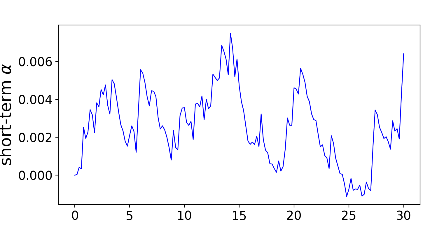
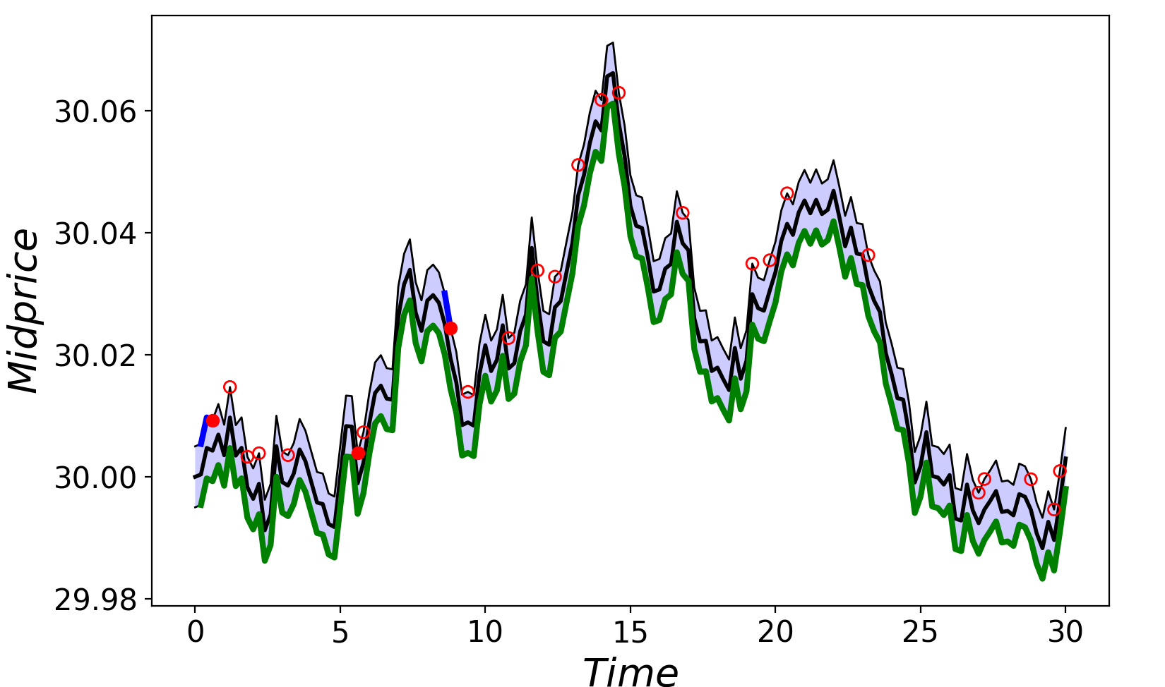
See simulation plots for the alpha process and midprice over the short time range of T = 30 seconds with dt = .2 seconds in Figures 3 and 4.
Acceleration results
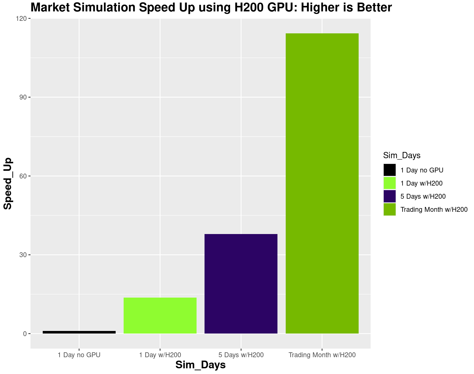
Performance results between the CPU and an NVIDIA H200 GPU for three simulation time ranges are shown in Figure 5. For long time ranges of one month, the acceleration is 114x, which takes advantage of the large number of CUDA cores of the NVIDIA H200 Tensor Core GPU. Using a robust number of simulations such as 1,000 allow mean and standard deviation midprice, alpha, and P&L to be computed.
The source of the speedup
The speedup provided by the GPU comes from the geometry of the algorithm being 2D. In the first dimension, time from 0 to the end T in seconds or fractions of seconds, there is no opportunity for GPU speedup because of the sequential nature of the stochastic differential equation time simulation. The stock price value at the time just past the time point called s_path(t+Δt) depends on s_path(t), the prior value, and this continues down the time line.
The second dimension is for Nsims = 1,000, the number of paths to compute for a robust simulation. In general, Monte Carlo simulations provide a better estimate of the distribution of the calculated random variable as the number of simulations grows. So, at 1,000 or more simulations and for longer periods of time, GPUs can be relied on to perform the massively parallel computation needed much faster than otherwise, making the runs much more efficient. This carries over to machine learning at the level of the limit order book as demonstrated in the 2022 and 2023 studies based on the machine learning classification approach of a 2018 study.
Conclusion
As for midprice processes in the past, the new best practice simulations for high-frequency limit order and market order processes follow the method described in the book Stochastic Calculus for Finance II. The number of processes, when examining the order book, is much more involved and goes with the higher level sophistication of the high frequency counterparty participants. For a discussion of how well the normal distribution and log returns model the actual price behavior of the market for Monte Carlo simulations, see the book Financial Analytics with R.
In-depth treatment provided by Algorithmic and High-Frequency Trading details the dynamic programming optimization goals. Extending this more complex simulation into trading days at subsecond granularity is difficult to compute on even a multicore CPU and, from the results presented in this post, is best accomplished using the acceleration provided by a GPU.
While this simulation generates its own market states, experience with the use of large order book data sets also requires GPU acceleration and that can be witnessed by the success of GPUs in the capital markets technology domain. To handle many traded securities across many exchanges world-wide in the back-testing simulation, multiple GPUs would be required.
Download and install RAPIDS to get started enabling GPUs for your data science workloads. Remember to install an NVIDIA driver and CUDA toolkit beforehand.
Download Numba to begin using the package to accelerate your Python programs. While CuPy can provide a straightforward conversion to GPU arrays, Numba provides more control on the dimensions of matrix parallelism so was best suited for the solution featured in this post.
Join us for NVIDIA GTC 2025 and check out the session AI for Safe and Efficient Trading in Electronic Markets [S72692].
