Entropy-Based Methods for Word-Level ASR Confidence Estimation

Once you have your automatic speech recognition (ASR) model predictions, you may also want to know how likely those predictions are to be correct. This probability of correctness, or confidence, is often measured as a raw prediction probability (fast, simple, and likely useless). You can also train a separate model to estimate the prediction confidence (accurate, but complex and slow). This post explains how to achieve fast, simple word-level ASR confidence estimation using entropy-based methods.

Overview of confidence estimation

Have you ever seen a machine learning model prediction and wondered how accurate that prediction is? You can make a guess based on the accuracy measured on a similar test case. For example, suppose you know that your ASR model predicts words from recorded speech with a Word Error Rate (WER) of 10%. In that case, you can expect that every word this model recognizes is 90% accurate.

Such a rough estimate may be enough for some applications, but what if you want to know with certainty which word is more likely to be correct and which is not? This will require using prediction information beyond the actual words, such as the exact prediction probabilities received from the model.

Using raw prediction probabilities as a measure of confidence is the fastest way to tell which prediction is more likely to be correct, which is less likely to be correct, and which is the simplest to implement.

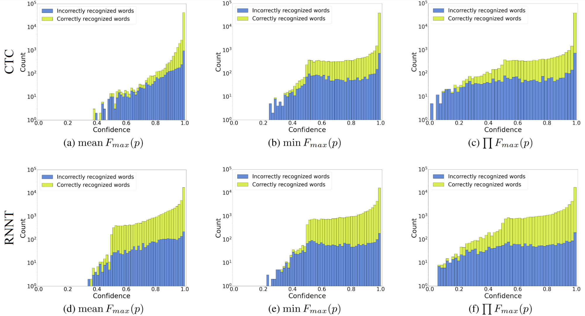
But are raw probabilities useful as confidence estimations? Not really. Figure 1, for example, is confidence computed for greedy search recognition results: frame by frame for linguistic units with the highest probability (“maximum probability” or $F_{max}(p)$ ) and then aggregated into word-level scores. What you can see there is called “overconfidence,” a feature of the model when its prediction probability distribution is skewed towards the best hypothesis.

In other words, the model almost always gives a probability close to one for one possible prediction and zero for any other. Thus, even if the prediction is incorrect, its probability will often be greater than 0.9. Overconfidence has nothing to do with the model’s architecture or its components: simple convolutional or recurrent neural networks can have the same overconfidence degree as transformer- or conformer-like models.

Overconfidence comes from the loss functions used to train end-to-end ASR models. Simple losses reach a minimum when the target prediction probability is maximized, and any others have zero probability. These include losses like the cross-entropy, ubiquitous connectionist temporal classification (CTC) or recurrent neural network transducer (RNN-T), or any other maximum likelihood family loss functions.

Overconfidence makes prediction probabilities unnatural. It is difficult to set the correct threshold separating correct and incorrect predictions, which makes using raw probabilities as confidence nearly useless.

Six log histograms of correctly and incorrectly recognized words against their confidence scores. Aggregation pushes confidence scores of incorrect words toward zero. However, these confidence aggregation functions do little to separate the distribution of correct predictions from incorrect ones: the shapes of correct and incorrect distributions mirror each other. — Figure 1. Stacked log histograms of correctly and incorrectly recognized words against their confidence scores. Subfigures (a) and (d) are obtained with the mean of the predictions of frames belonging to the same word, (b) and (e) with the minimum, and (c) and (f) with the product ( $\Pi$ ).

Figure 1. Stacked log histograms of correctly and incorrectly recognized words against their confidence scores. Subfigures (a) and (d) are obtained with the mean of the predictions of frames belonging to the same word, (b) and (e) with the minimum, and (c) and (f) with the product ( $\Pi$ ).

An alternative to using raw probabilities as confidence is to create a separate trainable confidence model to estimate confidence based on the probabilities and, optionally, ASR model embeddings. This approach can deliver fairly accurate confidence at the cost of training the estimator for each model, incorporating it into the inference along with the main model (and inevitably slowing the inference down), and lack of interpretability.

However, if you want the best possible measure of correctness and are comfortable with the system where a neural network estimates another neural network, try neural confidence estimators.

Entropy-based confidence estimation

This section features a non-trainable yet effective confidence estimation approach. You will learn how to make fast, simple, robust, and adjustable confidence estimation methods for CTC and RNN-T ASR models in the greedy search recognition mode.

A simple entropy-based confidence measure

Treating confidence simply as the raw prediction probability is a no-go, as explained above. Extending this definition to a function of all available knowledge on the interval [0,1] is preferable. Taking prediction probabilities “as is” falls under this definition. This approach enables you to experiment with adding external knowledge to the estimation or using the existing information (probabilities) in new ways.

Confidence must stay true to its primary purpose, which is to be a measure of correctness. At a minimum, it must behave as such: assign higher values to predictions that are more likely to be correct.

As a confidence measure, entropy is theoretically justified and works fairly well. In information theory, entropy is a measure of uncertainty, which calculates the uncertainty value based on probabilities of all possible outcomes.

This is exactly what is needed for ASR with the greedy decoding mode, where there is only one prediction per probability vector. Simply assign the entropy value to the prediction. Then invert the entropy value (to make it “certainty”) and normalize it (map it to [0,1]), as shown below.

$F_{g}(p) = 1 - \frac{H_{g}(p)}{\max H_g(p)} = 1 + \frac{1}{\ln V } \sum p_v \ln(p_v)$

$H_g(p)$ is the Gibbs entropy (which is more convenient than the Shannon entropy when dealing with natural logarithmic probabilities), $V$ is the number of possible predictions (vocabulary size for ASR models), and $F_{g}(p)$ is the Gibbs entropy confidence. Note that if the model is completely unsure (all probabilities are 1/ $V$ ), confidence will be zero even if there is still a 1/ $V$ chance of guessing the prediction correctly.

This normalization is convenient because it does not depend on the number of possible functions and gives you a simple rule of thumb: accept those close to one, discard those close to zero.

Advanced entropy-based confidence measures

The entropy-based confidence estimate above is quite applicable in that form, but there is still room for improvement. While theoretically correct, it will never show values close to zero (when all probabilities are equal) in practice due to the model’s overconfidence.

Moreover, it cannot address different degrees of overconfidence in this form. The second issue is tricky, but the first can be solved with a different normalization. Exponentiation will help here. When a negative number is raised to a power, the result will lie in the interval [0,1] and close to zero for most arguments.

With this property, you can normalize entropy using the following formula:

$F^{e}_{g}(p) = \frac{e^{-H_{g}(p)} - e^{-\max H_{g}(p)}}{1 - e^{-\max H_{g}(p)}} = \frac{V \cdot e^{(\sum p_v \ln(p_v))} - 1}{V - 1}$

$F^{e}_{g}(p)$ is the exponentially normalized Gibbs entropy confidence.

To make entropy-based confidence truly robust to overconfidence requires a method called temperature scaling. This method multiplies log-softmax by a number 0< $T$ <1. It is often applied to raw prediction probabilities to recalibrate them, but it does not significantly improve confidence. Applying temperature scaling to entropy is non-trivial: your entropy ceases to be entropy at certain values of $T$ . Specifically, unless the following inequality holds, the entropy cannot be normalized by the formula above. The maximum entropy will not be at the point where all probabilities are equal.

$\frac{1}{ln(V)} \leq T \leq \frac{1}{ln(\frac{V}{V-1})}$

The right side of the inequality is always true for $T$ , but the left side imposes restrictions. For example, if $V$ =128, then you cannot go below $T$ =0.21. It is tedious to keep this limitation in mind, so I advise you not to use regular entropy with temperature scaling.

Fortunately, you do not have to put temperature into entropy yourself. A few parametric entropies were introduced in the twentieth century. Among them are Tsallis entropy in statistical thermodynamics and Rényi entropy in information theory, which will be considered below. Both have a special parameter $\alpha$ , called entropic-index, which works like temperature scaling at 0< $\alpha$ <1. Their exponentially normalized confidence formulas look like this:

$F^{e}_{ts}(p) = \frac{e^{\frac{1}{1 - \alpha} (V^{1 - \alpha} - \sum p_v^{\alpha})} - 1}{e^{\frac{1}{1 - \alpha} (V^{1 - \alpha} - 1)} - 1}$

$F^{e}_{r}(p) = \frac{V \bigl(\sum p_v^{\alpha}\bigl)^{\frac{1}{\alpha - 1}} - 1}{V - 1}$

$F^{e}_{ts}(p)$ and $F^{e}_{r}(p)$ are the Tsallis and Rényi confidence measures, respectively. Note that the Rényi exponential normalization is performed with base 2 to match the logarithm and simplify the formula. These confidence measures may seem intimidating, but they are not difficult to implement and almost as fast to calculate as the maximum probability confidence.

Confidence prediction aggregation

So far, this post has considered the confidence estimation for a single probability vector or for a single frame. This section shows a full-fledged confidence estimation method for word-level predictions, introducing prediction aggregation.

Entropy-based confidence can be aggregated in the same way as the maximum probability: with the mean, minimum, and the product of frame predictions belonging to the same word. Regardless of the measure, two questions must be answered when aggregating ASR confidence predictions: 1) how to aggregate predictions to linguistic units versus linguistic units to words, and 2) what to do with so-called <blank> frames (frames on which the <blank> token was predicted). As before, the first question is simple, and the second question is tricky.

RNN-T models emit only one non-<blank> token each time it occurs, so you can simply take this prediction as unit-level confidence and put it to the word confidence aggregation. CTC models can repeatedly emit the same non-<blank> token while the corresponding unit is pronounced. I found that using the same aggregation function for units as for words is good enough, but overall there is room for experimentation.

There are two ways to handle <blank> frames for confidence aggregation: use them or drop them. While the first option looks natural, it forces you to figure out exactly how to assign them to the nearest non-<blank> unit.

You can put them with the closest left unit, just the closest unit, or something else, but it is better to drop them. Why? Aside from being easier this gives (surprisingly) better results for the advanced entropy-based measures. It is also more theoretically justified: <blank> predictions contain information about units and words that were not recognized while spoken (so-called deletions). If you try to incorporate <blank> confidence scores into the aggregation pipeline, you will likely contaminate your confidence with information about deleted units.

Evaluation results and usage tips

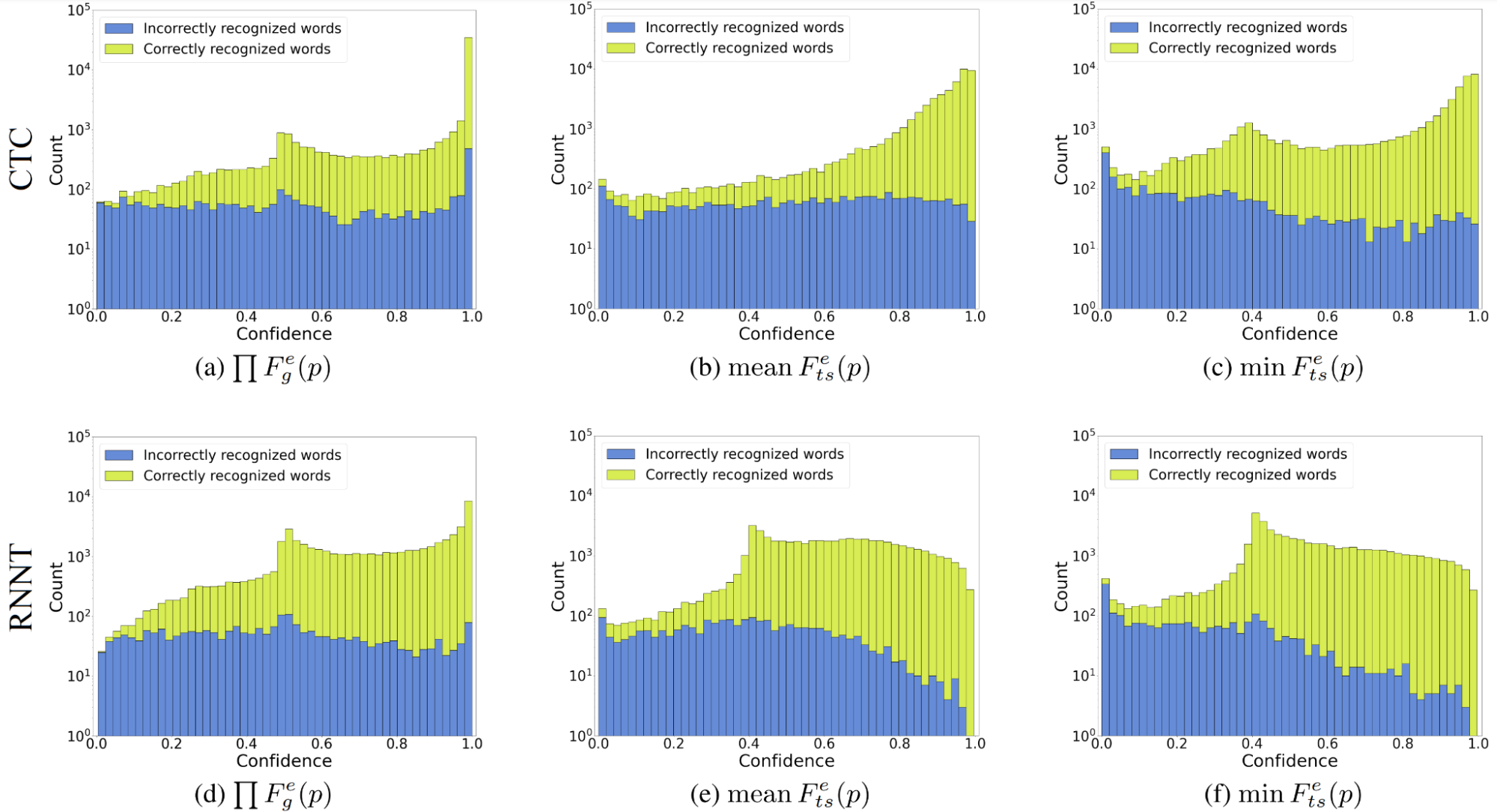
Now, see if the proposed entropy-based confidence estimation methods are better than the maximum probability confidence. Figure 2 may resemble Figure 1 with the maximum probability confidence distributions, but you can see that the entropy-based methods transform correct and incorrect word distributions for their better separation. (Different distribution shapes indicate better separability.)

All three methods cover the entire confidence spectrum. Even though the product aggregation performed best for the exponentially normalized Gibbs entropy confidence, this entropy itself does not handle overconfidence well. Tsallis entropy-based confidence with $\alpha$ =1/3 performed well with both mean and minimum aggregations. However, I prefer the minimum because it minimizes confidence for incorrect words more intensively. Overall, the exponential normalization gives full coverage of the confidence spectrum, and advanced entropy is better than simple.

CTC and RNN-T predictions for the exponentially normalized Gibbs entropy-based confidence estimation method with product aggregation are slightly overconfident with the uniform incorrect word distribution and the trend of correct words to confidence score 1. For CTC, the exponentially normalized Tsallis and entropy-based method with mean aggregation pushed correct words towards 1, keeping incorrect words distributed uniformly. For RNN-T, the method pushed incorrect words towards 0, holding the correct ones on a plateau from 0.4 to 1. The exponentially normalized Tsallis entropy-based method with minimum aggregation minimized confidence for incorrect words more intensively than the mean-aggregated method. — *Figure 2. Stacked log histograms of correctly and incorrectly recognized words against their confidence scores as in Figure 1, but for different confidence estimation methods*

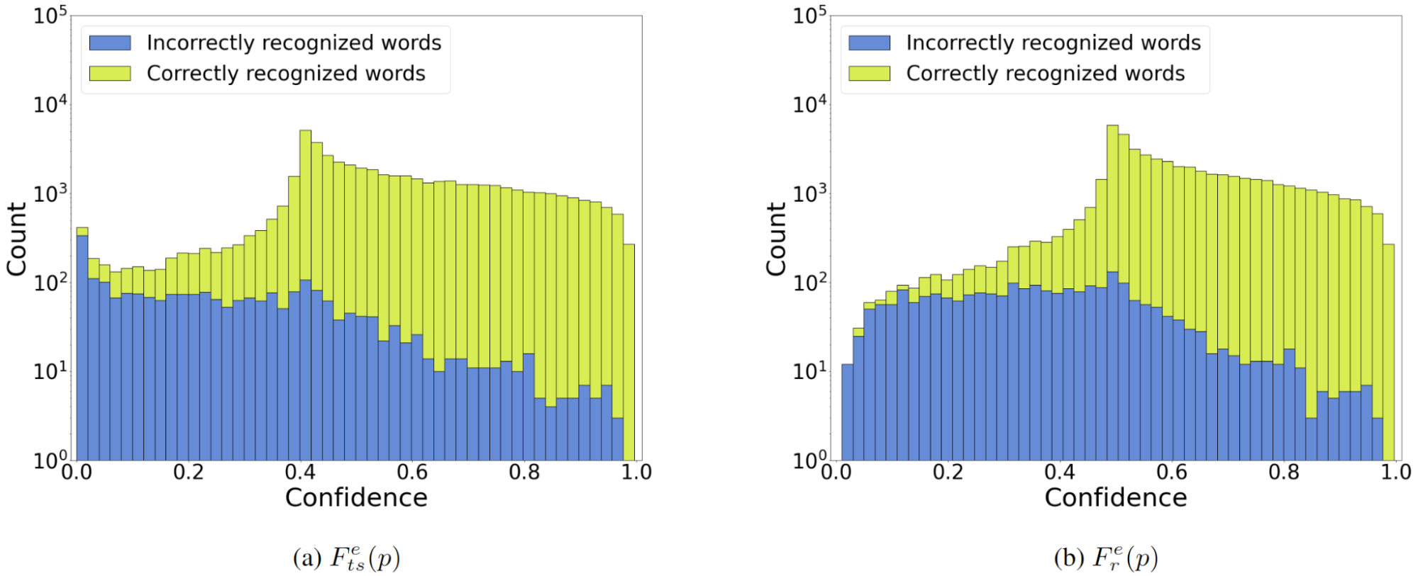
Where is the Rényi entropy in the comparison? Tsallis- and Rényi-based methods perform almost identically despite the visible difference in their formulas (Figure 3). For the same $\alpha$ and aggregation, Tsallis entropy gives a slightly stronger distribution separation at the price of the shifted peak of the correct distribution. I like the Tsallis-based confidence method more, but it is quite possible that Rényi might be better for your particular case, so I suggest trying both.

Two similar log-histograms of correctly and incorrectly recognized words against their confidence scores. The left one is for the Tsallis entropy-based method and the right one is for the Rényi. On the left histogram, the incorrect word distribution peaks at confidence 0, a plateau from 0 to 0.4, and a gentle slope from 0.4 to 1. The correct word distribution increases sharply from 0 to a peak at 0.4, after which it plateaus to 1. On the right histogram, both distributions have peaks at 0.5, and all other properties are similar to the left histogram. — *Figure 3. Comparison between Tsallis and Rényi entropy-based confidence estimation methods for the RNN-T model and $\alpha$ =1/3*

A final question is how to choose $\alpha$ . The answer depends on the overconfidence of the ASR model (the stronger the overconfidence, the smaller $\alpha$ should be) and what result you want to achieve. Set your $\alpha$ small enough to achieve the best distribution separability (Figure 4).

If you are willing to sacrifice the naturalness of the scores (getting reasonably high confidence scores for correct predictions) for better classification capabilities, you should opt for a smaller $\alpha$ .

Three similar log-histograms of correctly and incorrectly recognized words against their confidence scores. From left to right, they correspond to alpha values ½, ⅓, and ¼. The left histogram has two peaks near 0.4 and 1 for the correct word distribution and a plateau between them. The incorrect distribution also has a peak near 0.4, a plateau from the left, and a gentle slope from the right. The center and the right histograms are very much alike, with only two differences: the incorrect distribution of the right histogram does not reach 1, while the correct distribution has a flatter slope from 0.4 to 0. — *Figure 4. Comparison between different $\alpha$* *values for the Tsallis entropy-based method with the RNN-T model*

What remains is to mention the formal evaluation of the proposed entropy-based methods. First, entropy-based confidence estimation methods can be four times better at detecting incorrect words than the maximum probability method. Second, proposed estimators are noise robust and allow you to filter out up to 40% of model hallucinations (measured on pure noise data) at the price of losing 5% of correct words under regular acoustic conditions. Finally, entropy-based methods gave similar metrics scores for CTC and RNN-T models. This means that you can use confidence scores from RNN-T model predictions, which was not practical before.

Conclusion

This post provides three main takeaways:

Use Tsallis and Rényi entropy-based confidence instead of raw probabilities as measures of correctness for ASR greedy search recognition mode. They are just as fast and much better.
Tune the entropic index $\alpha$ (the temperature scaling analog for entropy) on your test sets. Alternatively, you can just use 1/3.
Try your own ideas to find even better confidence measures than entropy.

For detailed information on the evaluation of the proposed methods, see Fast Entropy-Based Methods of Word-Level Confidence Estimation for End-To-End Automatic Speech Recognition by Aleksandr Laptev and Boris Ginsburg.

All methods, as well as evaluation metrics, are available in NVIDIA NeMo. Visit NVIDIA/NeMo on GitHub to get started.