Discovering GPU-friendly Deep Neural Networks with Unified Neural Architecture Search

After the first successes of deep learning, designing neural network architectures with desirable performance criteria for a given task (for example, high accuracy or low latency) has been a challenging problem. Some call it alchemy and some intuition, but the task of discovering a novel architecture often involves a tedious and costly trial-and-error process of searching in an exponentially large space of hyper-parameters. The goal of neural architecture search (NAS) is to find novel networks for new problem domains and criteria automatically and efficiently.

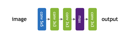
UNAS searches the best models on DGX station. The discovered models can be further optimized by TensorRT on target devices. — *Figure 1. An overview of UNAS training and deployment on the target devices.*

In the simplest form, NAS is the problem of choosing operations in different layers of a neural network. For example, for the image classification problem, the goal of NAS is to decide the best operations for each layer in a network under given conditions.

A small network is constructed by a stack of 5 different operations selected among 5x5 convolution, 3x3 convolution, and max pooling in blue, green and purple. Different colors represent different types of operations. — *Figure 2. The NAS goal is to find the best operations for each layer of a five-layer network. The operations are selected among 5×5 convolution, 3×3 convolution, and max pooling.*

Early work on NAS used reinforcement learning (RL) to obtain state-of-the-art performance on a variety of tasks. Although these methods are generic and can search for architecture with a broad range of criteria, they are often computationally demanding. For example, the approach proposed by Zoph et al. in Neural Architecture Search with Reinforcement Learning required about 22,400 GPU-hours on NVIDIA K40 GPUs. Recently, several differentiable NAS frameworks—such as DARTS: Differentiable Architecture Search —have shown promising results while reducing the search cost to a few GPU days. Although these methods complete the search much faster than the original RL-based methods, they have their own disadvantages.

In this post, we briefly review differentiable and RL-based NAS models and present a architecture search framework that bridges the gap between these two streams.

Differentiable NAS compared to RL-based NAS

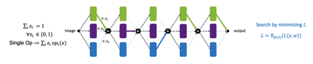
To better understand differentiable NAS, consider an example where you would like to choose operations for each layer of a five-layer network. The basic idea of differentiable NAS is to create a network by stacking mixed operations. In each mixed operation, you apply all the candidate operations in each layer and linearly combine their outputs. The mixing coefficients, $\zeta$ here, are designed to act as selection parameters.

In each mixed operation, the sum of weighted coefficients, zeta’s is one. The output of each mixed operation is the weighted sum of all the candidate operations in each layer. — *Figure 3. In differentiable NAS, a network is created by stacking mixed operations. ζ’s are continuous selection parameters.*

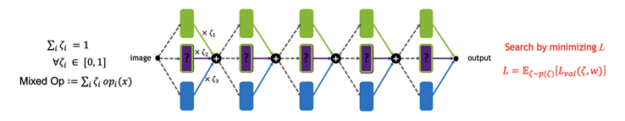
Because everything in this network is differentiable, you can perform an architecture search by minimizing a loss function such as cross-entropy loss. The minimization can be done with respect to both architecture parameters ζ as well as all the network parameters w. The final architecture is then created by choosing the operation that obtains the largest coefficient in each layer. There are different approaches to represent the coefficients. Here, consider SNAS, which uses the Gumbel-Softmax relaxation to represent the distribution over mixing coefficients. The main advantage is that the gradients can be estimated easily using the reparameterization trick.

The mixing coefficients in differentiable NAS are in fact a continuous relaxation of categorical one-hot selection parameters, z’s below, that select an operation per layer. Because these binary parameters are non-differentiable, early work in NAS used a more generic algorithm for training called REINFORCE. Like SNAS, in the RL-based NAS, you also search architecture by minimizing the expected value of a loss. However, because in this case the architecture selection parameters are binary, you only can use high-variance gradient estimators from RL.

The visualization of a deep network of RL-based NAS. Compared to Figure 2, you use one-hot binary selection parameters z in RL-based NAS to select an operation in each layer instead of mixing coefficients in differentiable NAS ranging from zero to one. — Figure 4. In RL-based NAS, search is done by minimizing the expected value of a loss with respect to a distribution over architecture parameters p(z), where z’s are one-hot binary selection parameters instead of continuous parameters ζ’s in differentiable NAS.

UNAS: The best of both worlds

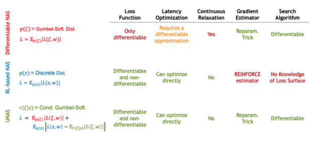
Differentiable NAS and RL-based NAS have their own advantages and disadvantages:

RL-based NAS can work with both differentiable and non-differentiable loss functions but differentiable NAS can only work with differentiable loss functions.
Because of this, for minimizing latency, differentiable NAS requires a differentiable approximation of latency.
RL-based NAS doesn’t introduce any continuous relaxation.
Differentiable NAS relies on the reparameterization trick which is less noisy and easier to train.
Differentiable NAS has access to the gradient information and it often converges faster.

The main question is whether you can have the best of both worlds. At CVPR this year, we introduced a novel NAS framework called UNAS that unifies RL-based NAS with differentiable NAS.

In this table, UNAS, the novel unified NAS framework, enjoys the advantages from both RL-based NAS and differentiable NAS. — *Figure 5. RL-based NAS and differentiable NAS are compared against each other for different criteria. UNAS offers the best of both worlds.*

The core idea of UNAS is to create two networks: one with one-hot selection parameters and the other with mixed operations as a control variate for variance reduction. Figure 6 shows that the coefficients of the mixed operations are sampled from a conditional Gumbel-Softmax distribution, which generates coefficients correlated with the one-hot parameters. This way UNAS optimizes the REINFORCE objective, and it uses the differentiable NAS for variance reduction.

The UNAS Loss contributed by the REINFORCE term from the first network, the SNAS term, and the Control Variate term from the second network. — Figure 6. In UNAS, we search for network architecture using the reinforcement learning objective and we use the differentiable NAS for variance reduction. We create two networks: one with one-hot selection parameters and one with mixed operations as a control variate for variance reduction.

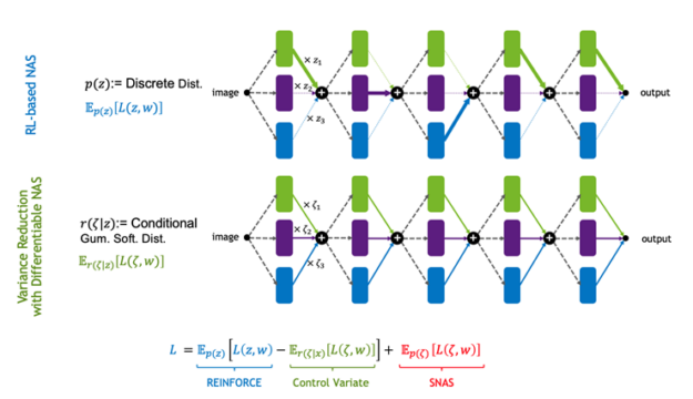
The main advantage of UNAS is that it is generic like RL-based NAS, but it is also gradient-based like differentiable NAS. It is easy to show that RL-based NAS and differentiable NAS are special cases of the objective.

Model benchmark

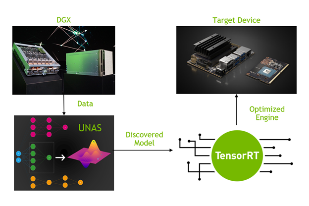
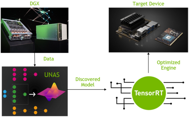
In the UNAS paper, we chose NVIDIA V100 GPUs as a target platform for deployment and searched for an image classification model. For more information about searching and training, see UNAS: Differentiable Architecture Search Meets Reinforcement Learning. For more information about the implementation of the UNAS algorithm, see the NVlabs/unas GitHub repo.

For a minimal effort to speed up the discovered model, use the NVIDIA Automatic Mixed Precision (AMP) library with FP16 support, which allows mixed precision for training and inference.

To obtain further speedups, use NVIDIA TensorRT SDK for high-performance inference. TensorRT-based applications can significantly accelerate inference on GPUs, thanks to its inference optimizer and runtime. In addition, TensorRT also provides optimizations for different precisions to further speed up inference with little or no accuracy drop.

To export the PyTorch pretrained model to the ONNX format, add a few lines after the UNAS model is constructed:

# First, create the UNAS model before exporting
model.eval() # put model in evaluation mode
input = torch.randn((1, 3, 224, 224))
input_names = [ "input" ]
output_names = ["output"]
torch.onnx.export(model, input, "model.onnx", opset_version=10, verbose=True, input_names=input_names, output_names=output_names)

To benchmark the latency of the model with TensorRT, use NVIDIA TensorRT container 20.07, which makes TensorRT 7.1.3.4, CUDA 11.0, and CUDNN 8.0.1 available. For more information, see the release notes. With the exported model stored in the current working directory, you can measure the inference latency in FP32 and FP16 precision with the following commands. The INT8 type on Tensor Cores is not supported on V100.

docker pull nvcr.io/nvidia/tensorrt:20.07-py3
docker run -it --gpus all --network=host --rm -v $PWD:/home/unas \
   nvcr.io/nvidia/tensorrt:20.07-py3
cd /home/unas
/workspace/tensorrt/bin/trtexec --onnx=model.onnx --avgRuns=100 -batch=32
/workspace/tensorrt/bin/trtexec --onnx=model.onnx --fp16 --avgRuns=100 -batch=32

Now, look at the inference speed. Figure 7 shows the comparisons of latency numbers between the original PyTorch implementation and TensorRT-accelerated models running on a V100 GPU with batch size 32.

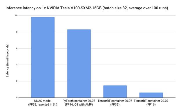
A bar chart of inference time comparison. The TensorRT optimization achieves 6X and 16X speedup in FP32 and FP16, respectively compared to the original models running in PyTorch. — *Figure 7. Inference time comparison between the PyTorch model and TensorRT-optimized model.*

Compared to the original PyTorch model in FP32, switching to FP16 with AMP reduces the latency from 9.8 ms to 8.3 ms. When TensorRT comes into play, the latency in FP32 is further reduced to 1.5 ms, which is more than a 6X speedup compared to the original model running in PyTorch. By enabling FP16 in TensorRT, latency can be further reduced to 0.6 ms, corresponding to a 16X speedup to the PyTorch latency in FP32 reported in the UNAS paper.

Hardware-aware search and latency estimation

One of the advantages in UNAS is the capability of handling non-differentiable loss functions (such as for penalizing high inference latency). To estimate latency for each architecture sample, a simple five layer, fully connected, neural network was trained on a few thousands of latency-architecture pairs measured in PyTorch. With this small neural network, you can estimate the latency of other networks on the fly while computing loss during search.

Another practical approach to estimating the latency of a network is to create a look-up table (LUT) of each candidate block, with the latency measured on the target hardware using compile-time optimizations (that is, TensorRT). In this case, the latency of a network can be estimated by adding up the latency of each candidate block/layer. This approach yields a searched model with more accurately estimated latency when deployed on NVIDIA platforms using TensorRT.

Conclusion

In this post, we briefly introduced the concept of NAS and presented a state-of-the-art method dubbed UNAS to find hardware-friendly models that run efficiently on NVIDIA GPUs. With the NVIDIA TensorRT library, you can accelerate model inference further.

We are currently developing tools and workflows for LUT creation and application to find optimal models on different target devices. In addition, we plan to show how to optimize models on more devices such as NVIDIA Jetson and NVIDIA DRIVE products. For more information, see our talk at GTC 2020: Automating DNN Design for NVIDIA DRIVE AGX: Platform-Aware Neural Architecture Search, which showcases applications of NAS in practice. Check out our NVlabs/UNAS repo and stay tuned!