
Magnetic resonance imaging (MRI) is a useful imaging technique for imaging soft tissue or molecular diffusion. However, scan times to acquire MR images can be quite long. There are several methods that can be used to reduce scan times, including rectangular field-of-view (RFOV), partial Fourier imaging, and sampling truncation. These methods result in either a decreased signal-to-noise ratio (SNR) or decreased resolution. For more information, see k-Space tutorial: an MRI educational tool for a better understanding of k-space.
The Gibbs phenomenon, also known as ringing or truncation artifacts, can appear in the resulting image when using sampling truncation technique to reduce scanning and data transfer time. Typically, the Gibbs phenomenon is removed by smoothing the image, resulting in decreased image resolution.
In this post, we explore a deep learning method with the NVIDIA Clara AGX developer kit to remove the Gibbs phenomenon and noise from MR images while maintaining high image resolution.
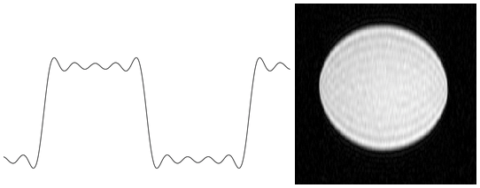
A signal can be represented as an infinite sum of sine waves of varying frequency and phase. MR images are approximated by using relatively few harmonics leading to the presence of Gibbs phenomenon. Figure 1 shows an analogous 1-dimensional situation of approximating a square wave with only a few harmonics, with the Gibbs phenomenon in an MRI phantom on the right.
Datasets and models
We extended the work of an existing deep learning method for Gibbs and noise removal, known as dldegibbs. For more information, see Training a Neural Network for Gibbs and Noise Removal in Diffusion MRI. The code for that whitepaper is in the /mmuckley/dldegibbs GitHub repo.
Approximately 1.3 million ImageNet images with simulated Gibbs phenomenon and Gaussian noise were used as training data in their work. In our project, we tested some of the pretrained dldegibbs models developed by Muckley et. al. and we trained our own models using the Open Images dataset. We finally tested different models with MRI diffusion data.
Why simulate the Gibbs phenomenon?
One benefit of using dldegibbs compared to other networks is that it does not require access to the raw MRI data and system parameters. This data is hard to obtain because storage requirements for this data are high and this data is typically not retained after image reconstruction.
Another benefit is that no proprietary information or signing of research agreements with vendors is required. Also, time is saved from collecting and distributing medical data, which can be challenging. Training the model with a heterogeneous dataset such as ImageNet or Open Images potentially enables application of this approach to other MRI sequences or imaging modalities because the training data is intrinsically object agnostic.
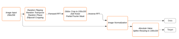
The data loaders of dldegibbs create two images for each loaded image: a training image and a target image. The training image gets created simulating the Gibbs phenomenon on the original image in the Fourier domain. The original image is resized and used as the target image. The data loaders include standard data augmentation methods (random flipping, cropping), followed by random phase simulation and ellipse cropping. Next, the FFT is applied to the original images, Gibbs cropping is performed, complex Gaussian noise is added, and partial Fourier is simulated. Finally, the inverse FFT is applied, and the images are normalized. Figure 2 shows the simulation pipeline.
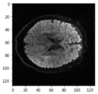
In this project, we used the Open Images dataset consisting of over 1.7 million training images. We then tested the trained models on an MRI diffusion dataset consisting of 170 patients (996424 axial slices) [5]. Figure 3 shows an example MRI diffusion slice.
Results
Figure 4 shows an example validation image tested with a dldegibbs model that was trained with the Open Images training dataset. Figure 5 shows the corresponding errors. The images for training were cropped in Fourier space from 256×256 to 100×100. No partial Fourier imaging was simulated in this model.
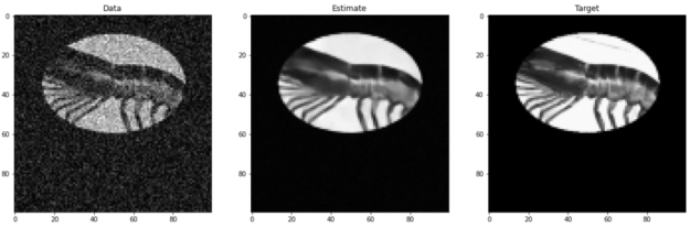
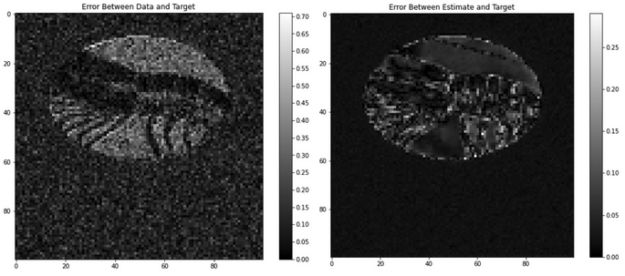
The average MSE between data and target is 13.2 ± 9.2%. The average error between estimate and target is 2.9 ± 2.7%. For this image, the dldegibbs model results in a greater than 10% improvement in quality of image.
Summary
In this post, we provided a solution that can be used with the Clara AGX development kit to remove noise and Gibbs phenomenon from MR images using the following resources:
- A commercially available dataset, known as Open Images
- An open-source ML model, known as dldegibbs
We’ll release the dldebiggs reference Docker container on NGC soon. To find all available containers, see the Clara AGX Collections.
