Autonomous vehicles (AV) are transforming the way we live, work, and play—creating safer and more efficient roads. In the future, every vehicle may be autonomous: cars, trucks, taxis, buses, and shuttles. AI and AV are transforming mobility and logistics, creating new business models and enormous efficiencies for the $10T transportation industry.
These revolutionary benefits require massive computational horsepower and large-scale production software expertise. NVIDIA has been working on self-driving cars for many years and has built an internal infrastructure with DGX systems and Mellanox networking capabilities, called NVIDIA DRIVE Infrastructure.
NVIDIA DRIVE Infrastructure is a complete workflow platform for data ingestion, curation, labeling, and training plus validation through simulation. NVIDIA DGX systems provide the compute needed for large-scale training and optimization of deep neural network models. These systems also provide compute needs for running replay and data factory operations. NVIDIA DRIVE Constellation provides physics-based simulation on an open, hardware-in-the-loop (HIL) platform for testing and validating AVs before they hit the road.
NVIDIA has introduced NVIDIA DGX A100, which is built on the brand new NVIDIA A100 Tensor Core GPU. DGX A100 is the third generation of DGX systems and is the universal system for AI infrastructure. Featuring five petaFLOPS of AI performance, DGX A100 excels on all AI workloads: analytics, training, and inference. It allows organizations to standardize on a single system that can speed through any type of AI task at any time and dynamically adjust to changing computing needs over time. This unmatched flexibility reduces costs, increases scalability, and makes DGX A100 the foundational building block of the modern AI data center.
NVIDIA DGX A100 redefines the massive infrastructure needs for AV development and validation. NVIDIA has outlined the computational needs for AV infrastructure with DGX-1 system. In this post, I redefine the computational needs for AV infrastructure with DGX A100 systems.
Data center requirements for AV are driven by mainly: data factory, AI training, simulation, replay, and mapping. This post introduces details about data factory, AI training and replay, and the scale for DGXA100 systems. Mapping also requires computing infrastructure similar to AI training, so this is not explicitly discussed in this post.
AV: Massive amounts of data
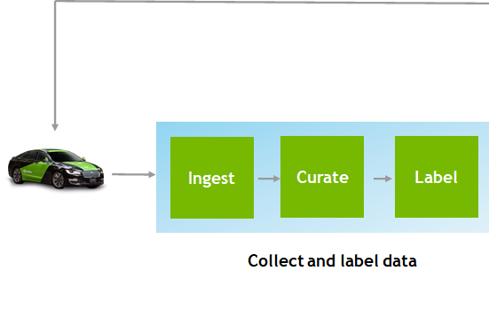
Each data-collection car generates upwards of two petabytes of data with billions of images per year. The data center uses inferencing to ingest, curate, and annotate this data for use in the AI model training.
You need an optimized workflow and infrastructure to manage the data pipeline for data ingestion from vehicles: computing resources for transcoding and compression; labeling services; a centralized geo-distributed data lake and repository for the storage and retrieval of all AV data, including raw sensor data; data annotation and curation; ground-truth data used in training and testing models; performance metrics on replay and simulation; and trained models.
Obviously building AI-powered, self-driving cars requires a massive data undertaking. The amount of data depends on the following factors:
- The size of the data campaign fleet
- Geographic and regional dispersion of the fleet
- The number and types of sensors used in the data-collection vehicle
- The car data campaign operation hours
- The percentage of useful and diverse data
- Data compression techniques
Building and operating a data-collection vehicle is expensive, so organizations generally build only a few data-collection cars. They also rely on data collected by consumer cars. In general data, a campaign fleet ranges between 5-50 cars.
A data-collection vehicle uses multiple sensors, mainly cameras, radar, and lidar. Data is collected to build AI that helps with the driving of the car as well as driver monitoring and assistance.
Data-collection cars typically use 6-10 cameras, 4-6 radars, and 2-4 lidars of different resolutions and range. For this post, I focus on data generated by cameras in cars, as that dominates the overall data collection. On average, these collection cars drive 8 hours/day for 250 days/year, which is 2,000 hours/year/car. With two 8-hour shifts, it results in 4,000 hours/year/car.
Collection vehicles are traditionally sensor-robust compared to a vehicle validation fleet. Their recording frequency and resolution can be higher, compared to production cameras, to validate optical technics. Downsampling is used to bring different sensor setups in line. Being greedy on the data collected (for example, sampling a wider array of CAN and bus signals) allows for the cross validation of different sensors and plausibility checks.
However, not all collected data is useful. Collected data can get corrupted because of faulty sensors, dust on the camera lens, faulty mounting of sensors, and so on. Then there are the questions of data integrity and the lack of diverse information in collected data. In my experience, useful data is a much smaller subset of the total collected data. On average, I find only 30–50% of data is useful. A preprocessing tier placed in closer proximity to data collection can influence data volume transfers and provide a differentiation mechanism to elevate data value.
Data storage depends on the amount of data collected and how it is stored. You can apply lossless or lossy compression to data and choose data to store for the long term. I revisit the storage requirements later in this post.
Table 1 shows a typical range of data storage requirements for a car fleet ranging from 5–50 cars with 5–10 sensors (with a mix of 2.3 and 8 MPix cameras) and assuming 40% of collected data was useful. All numbers are converted into the nearest integer. This is directional guidance to understand the amount of the data generated by data-collection vehicles. You can refine the requirements based on your individual use case.
| Cars | Sensors | Image size (MB) | Collection hours/year/car | Uncompressed raw collected data (PB) | Uncompressed useful data (PB) |
| 5 | 5 | 2.3 | 2000 | 12.5 | 5 |
| 50 | 10 | 8 | 4000 | 1728 | 691 |
It is not necessary to label 100% of the collected data, as significant redundant information is collected that does not help to increase the accuracy of AI models. The best practice is to only label a downsampled dataset. Labeling is a costly, manual process. As your dataset grows, you need more intelligent ways to downsample the raw data. A simple approach typically used is to mine the collected raw data with pretrained AI models on deep neural networks (DNNs).
The downsampling process uses AI inferencing of the raw data using AI models. As these models continue to be improved during the AV development process, you must re-inference the entire dataset regularly with the most recent models. Assuming frequent updates of AI models, you might use an average of 2,500–5,000 hours of data every day for mining. This data keeps on increasing over time.
When you are inferencing an average of 2,500–5,000 hours of driving data with 10 sensors in a car on 10 AI networks with a turnaround time (TAT) of five days, you need 15-30 DGX A100. The simple formula used for computation is as follows:
# DGX A100 = ((# of Images (frames) / DGX inference throughput) x # of DNNs)/ TAT
Data mining changes based on the total amount of data collected and how often you must run the mining on the entire dataset. One example of compute requirements for data mining using camera data in a data factory is shown here. Each image is 2.3 MB. The formula to compute number of frames is as follows:
# Images / Year = # of Vehicles x # of Cameras x # of frames / second x # hours driven per year per car
| Fleet vehicles | Cameras per car | Frames per second | Hours driven per year | Dataset frames (B) | AI models | TAT (days) | DGX A100 total | |
| Scenario 1 | 5 | 5 | 30 | 2000 | 5 | 10 | 30 | 6 |
| Scenario 2 | 25 | 10 | 30 | 2000 | 54 | 10 | 60 | 28 |
| Scenario 3 | 50 | 16 | 30 | 2000 | 173 | 10 | 120 | 44 |
AI model training
In a typical AV development, you would develop 10 or more AI networks used for perception and in-car monitoring. Each network requires the training of an AI model on a labeled dataset. Datasets and DNNs are grown and developed incrementally, each new phase requiring research, exploration, and therefore computational resources.
Traditionally, published DNNs in collection fleets have a real-time, time-critical response while data-center–based scenario approaches offer increased complexity and fidelity to discovered the undetected. Figure 1 shows the workflow for each of these networks.
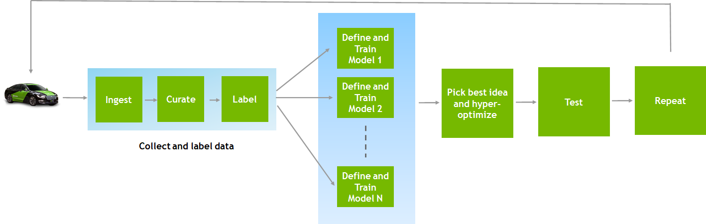
As shown in Figure 1, ingested data from data-collection cars is curated and labeled. Next, the AI network architecture is defined, and training jobs are run on labeled data. You pick the best idea for a given network and fine-tune the hyperparameters. Trained and fine-tuned models are tested with validation data. This feedback then goes to a data-collection campaign and new data is collected. The entire AI training process is an iterative process.
AI model training infrastructure sizing depends on multiple factors:
- Labeled images—The previous section illustrated the guidance on the amount of raw data collected by data-collection cars. With one car generating 2000 hours of data and considering five cameras per car running at 30 FPS, the total images can be calculated at 2,000 hours/year x 3,600 seconds/hour x 30 frames/second x 5 cameras = 1 billion images/year/car. As discussed earlier, 100% of collected data is not useful and labeling needs further downsampling. On average, downsampling data by taking one frame every 10 seconds gives a labeled data set of approximately three million images.
- TAT—This is an important factor to determine the size of the AI infrastructure. A larger TAT affects the productivity of AI engineers and data scientists, while a small TAT results in massive AI infrastructure. It is essential to choose the right TAT for training.
- Parallel experiments—For each AI model, you typically want to run
AI model development consists of mainly three phases: exploration, development, and model deployment.
Exploration phase
During the exploration phase, AI models are trained on smaller datasets (10–20K images), but many parallel experiments are performed. The reason for a higher number of parallel experiments is to test multiple architectures and methodologies to build AI networks. The exploration phase needs a small TAT (~1-3 hours) so that many parallel experiments can be performed in a day and AI engineers can be productive.
Development phase
The development phase down-selects a few AI models from the exploration phase and runs the training on a larger dataset (~200–300K frames). This phase typically needs a TAT of 24 hours as AI engineers run the models and go back home before resuming work. The number of parallel experiments is also lower compared to the exploration phase.
Model deployment phase
Model selection is not done frequently as this requires searching over the entire space of hyperparameters and running the training on a full dataset to fine-tune the AI models. The TAT is much larger (~5-10 days) based on the need for the release of models.
Discovering the undetected within published DNNs is critical for determining the overall robustness. DNNs are scored against a portfolio of tricky images and scenarios to evaluate abnormal road encounters, such as pedestrians, ladders, or mattresses on the highway. The TAT is roughly small depending on the level of unique corner cases provided. Sensitivity to sensor calibration also can be observed especially within the region over overlapping cameras with different pixel fidelity as in wide angle versus narrow field of view cameras and determining which field has an effective useful range before switching sensor suite.
Observe the sensitivity to sensor calibration, especially within the region of overlapping cameras with different pixel fidelity. Consider wide-angle compared to narrow-field-of-view cameras and determine which field has an effective useful range before switching sensor suites.
On average for all three phases, you run 10 parallel experiments every day with a 24-hour TAT target. Benchmarking reveals that, on average, it takes 24 hours to run training with 300K images on one DGX-1. With this, you can summarize as follows:
10 AI models x 10 parallel experiments x 1 DGX/Model/Exp = 100 DGX-1s to support the AV team today, with a total labeled dataset of ~ 3M (300K per AI model).
A100 provides 10-20x of peak performance improvement over V100 for AI training because of new architectural features introduced. On an AV AI training workload, the DGX A100 typically provides ~3x-5x improvement, as seen with benchmarking. For a conservative approach for infrastructure sizing and providing directional guidance, I consider 3x as an average performance improvement over DGX-1 systems. This means to run 10 AI models with 10 parallel experiments on labeled images dataset of 300K per AI model, you need approximately 35 DGX A100s with a TAT of 1 day.
| Labeled images (average) | AI models | Parallel experiments | TAT (days) | DGX A100 total | |
| Scenario 1 | 300,000 | 10 | 10 | 1 | 34 |
| Scenario 2 | 300,000 | 15 | 25 | 1 | 125 |
| Scenario 3 | 300,000 | 20 | 50 | 1 | 334 |
Table 3. Range sizing based on varying levels of maturity for AI for AV training.
The formula to compute the number of DGX A100 needed is as follows:
#DGX A100 = ((Avg. # Images per DNN / DGX-A 100 throughput x # AI models x # Parallel experiments)/TAT
The DGX A100 needs are driven not just by dataset size but also by how much you want to be exploring in parallel and how short your turnaround time is.
In the future, datasets will continuously expand with more data campaigns and more labeling capabilities. Compute scaling with larger data size is not linear. With dataset growth, the AV team does a lot of experimentation and research on downsampled datasets (downsized by 2 to 5x). Only production AI models, deployed with much larger TAT, go through the full data sets during training. Because of larger TAT, there is a smaller effect on compute sizing.
Replay
Replay is the process of replaying previously recorded sensor data from collection vehicles driving on-road against AV software. The replay is extremely useful for testing against a large body of real-world data. New DNNs are tested for improvements with regressions against annotated images collected from millions of driven miles.
The key reason to run replay is to do validation testing at scale in one of two modes:
- In HIL mode, you run
- In software-in-the-loop (SIL) mode, you can run these driving algorithms on a datacenter GPU to run at super real-time to do testing at scale.
The replay sizing depends on the following factors:
- Number of hours of data to be replayed
- TAT
- Parallel experiments
- Driving software pipeline
Driving software mainly consists of perception, path planning, control and vehicle dynamics, and control. This pipeline is different for everyone who is building AV software. The bottleneck in the pipeline determines the infrastructure sizing of the replay workload. Here are some examples:
- The driving pipeline is AI-heavy and most of the computing needs are for inference. This pipeline is bottlenecked by the inference workload.
- Another pipeline needs decoding of compressed data. It may be bottlenecked by the decoder throughput on the GPU.
- A replay pipeline may be bottlenecked by your CUDA performance.
Here is a sizing example, assuming that the replay workload is mostly dominated by inference. In this example, replay testing at scale runs a minimum of 10,000 hours of sensor data and can scale up to 100,000 hours or more of sensor data.
The total number of frames coming from sensors can be computed as follows:
#Frames = hours of validation * frames per hour
The compute needed from DGX A100 can be computed as follows:
#DGX A100 = (# frames* #parallel experiments)/TAT
| Validation hours for replay | Dataset frames (B) | Parallel experiments | TAT (days) | DGX A100 total | |
| Scenario 1 | 25,000 | 2.7 | 10 | 5 | 24 |
| Scenario 2 | 50,000 | 5.4 | 10 | 5 | 48 |
| Scenario 3 | 75,000 | 10.8 | 10 | 5 | 95 |
Summary
Developing AV is a computationally intensive problem and requires massive accelerated computing infrastructure. AV development begins with a data factory with petabytes of storage for the billions of sensor images generated from data-collection fleets and DGX A100 to preprocess the raw data and select images for labeling. An even larger number of DGX A100 are required to train and validate the AI models. Directional guidance is provided to size the AV infrastructure requirements for data mining, AI training, replay, and other workloads.
DGX A100 is a universal AI platform that allows you to run workloads in a scale-up as well as scale-out manner. It sets a new bar for compute density, packing five petaFLOPS of AI performance into a 6U form factor. It replaces legacy infrastructure silos with one platform for every AI workload.
DGX POD is the combination of NVIDIA accelerated compute architecture, Mellanox network fabric, and system management software. It delivers a solution that democratizes supercomputing power, making it readily accessible, installable, and manageable for AV infrastructure needs.
