
In this three-part series, you discover how to use NVIDIA Nsight Compute for iterative, analysis-driven optimization. Part 1 covers the background and setup needed, part 2 covers beginning the iterative optimization process, and part 3 covers finishing the analysis and optimization process and determining whether you have reached a reasonable stopping point.
Nsight Compute is the primary NVIDIA CUDA kernel-level performance analysis tool. It is part of the NVIDIA Nsight family of tools for GPU computing. For thorough introductions to the NVIDIA Nsight family profiler tools, see the following posts:
- Migrating to NVIDIA Nsight Tools from NVVP and Nvprof
- Transitioning to Nsight Systems from NVIDIA Visual Profiler / nvprof
- Using Nsight Compute to Inspect your Kernels
These posts point out that the GPU code performance analysis process usually begins with Nsight Systems. Eventually, the analysis may select a specific kernel to focus on, for further analysis using Nsight Compute. In this post, I discuss how Nsight Compute facilitates analysis-driven optimization (ADO) of GPU kernels.
ADO is predicated on the idea that making the most efficient use of your time involves focusing on the most important limiters to code performance, in pareto order. In a cyclical process, you want the tool to identify the current most important limiter to performance and, to the fullest extent possible, give you some clues about how to address it. The most important limiter to performance is the code characteristic that, if modified, would yield the largest improvement in performance.
Start by focusing on the fixes that yield the largest performance improvements. In a cyclical fashion, you use the tool to identify these areas, make code changes, and then use the tool again to assess the impact of these changes and identify the next area to look at. The process completes when you either run out of time or have identified, perhaps through some calculations, that further optimization is unlikely to yield significant performance improvement.
To follow along with this post, I recommend using CUDA 11.1 and Nsight Compute 2020.2 or newer. Several kinds of profiler output reviewed in this post may not be present if you use a previous version of the tool.
Code for analysis
You’re going to analyze code that is more complicated than my previous post on Nsight Compute. This code has multiple steps and phases to it. Using ADO, you go through a set of steps that successively improves the performance of the code by uncovering, in each step, a performance limiter. For more information about an additional example, see the Summary section.
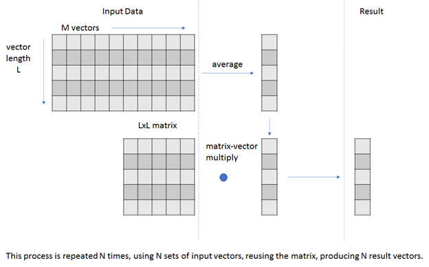
Use the performance limiter to guide your attempt to improve performance. The code that you analyze has two major phases:
- Average a set of vectors, producing a single average vector.
- Perform a matrix-vector multiply on the average vector, producing a result vector.
This code repeats these steps on different sets of incoming vectors but uses the same matrix to produce a set of result vectors. The starting point for this code was a CPU algorithm using OpenMP for parallelism that has been ported to a GPU version to achieve higher performance.
// compile with: nvcc -Xcompiler -fopenmp -o t5 t5.cu -O3 -lineinfo
#include
#include

#define cudaCheckErrors(msg) \
  do { \
    cudaError_t __err = cudaGetLastError(); \
    if (__err != cudaSuccess) { \
        fprintf(stderr, "Fatal error: %s (%s at %s:%d)\n", \
            msg, cudaGetErrorString(__err), \
            __FILE__, __LINE__); \
        fprintf(stderr, "*** FAILED - ABORTING\n"); \
        exit(1); \
    } \
  } while (0)


#include
#include <sys/time.h>
#define USECPSEC 1000000ULL

unsigned long long dtime_usec(unsigned long long start){

  timeval tv;
  gettimeofday(&tv, 0);
  return ((tv.tv_sec*USECPSEC)+tv.tv_usec)-start;
}

// perform vector averaging over M vectors of length L,  followed by matrix-vector multiply
// repeat the above N times
// input vectors are stored as a set of N column-major matrices
// for each k in N: output[k] = matrix*input[k]
template
void cpu_version1(T *input, T *output, T *matrix, int L, int M, int N){
#pragma omp parallel for
  for (int k = 0; k < N; k++){      // repeat the following, N times
    std::vector v1(L);           // vector length of L
    for (int i = 0; i < M; i++)     // compute average vector over M input vectors
      for (int j = 0; j < L; j++)
        v1[j] += input[k*M*L+j*M+i];
    for (int j = 0; j < L; j++)
      v1[j] /= M;
    for (int i = 0; i < L; i++)     // matrix-vector multiply
      for (int j = 0; j < L; j++)
        output[i*N+k] += matrix[i*L+j]*v1[j];
  }
}

const int my_L = 1024;
const int my_M = 1024;
const int my_N = 1024;

template
__global__ void gpu_version1(const T * __restrict__ input, T * __restrict__ output, const T * __restrict__ matrix, const int L, const int M, const int N){

  __shared__ T smem[my_L];
  size_t idx = ((size_t)blockIdx.x)*blockDim.x + threadIdx.x;
  for (int k = 0; k < N; k++){  // iterate over N data sets
    T v1 = 0;
    for (int i = 0; i < M; i++) // perform vector averaging
      v1 += input[k*M*L+idx*M+i];
    v1 /= M;
    for (int i = 0; i < L; i++){ // perform matrix-vector multiply
      __syncthreads();
      smem[threadIdx.x] = v1 * matrix[i*L+idx];
      for (int s = blockDim.x>>1; s > 0; s>>=1){
        __syncthreads();
        if (threadIdx.x < s) smem[threadIdx.x] += smem[threadIdx.x+s];}
      if (!threadIdx.x) output[k+i*N] = smem[0];}
  }
}

typedef float ft;

int main(){
  ft *d_input, *h_input, *d_output, *h_outputc, *h_outputg, *d_matrix, *h_matrix;
  int L = my_L; int M = my_M; int N = my_N;
  // host allocations
  h_input   = new ft[N*L*M];
  h_matrix  = new ft[L*L];
  h_outputg = new ft[N*L];
  h_outputc = new ft[N*L];
  // data initialization
  for (int i = 0; i < N*L*M; i++) h_input[i] = (rand()&1)+1;  // 1 or 2
  for (int i = 0; i < L*L; i++) h_matrix[i]  = (rand()&1)+1;  // 1 or 2
  // create result to test for correctness
  unsigned long long dt = dtime_usec(0);
  cpu_version1(h_input, h_outputc, h_matrix, L, M, N);
  dt = dtime_usec(dt);
  std::cout << "CPU execution time: " << dt/(float)USECPSEC << "s" << std::endl;
  // device allocations
  cudaMalloc(&d_input, N*L*M*sizeof(ft));
  cudaMalloc(&d_output,  N*L*sizeof(ft));
  cudaMalloc(&d_matrix,  L*L*sizeof(ft));
  cudaCheckErrors("cudaMalloc failure");
  // copy input data from host to device
  cudaMemcpy(d_input,  h_input,  N*L*M*sizeof(ft), cudaMemcpyHostToDevice);
  cudaMemcpy(d_matrix, h_matrix,   L*L*sizeof(ft), cudaMemcpyHostToDevice);
  cudaMemset(d_output, 0, N*L*sizeof(ft));
  cudaCheckErrors("cudaMemcpy/Memset failure");
  // run on device and measure execution time
  dt = dtime_usec(0);
  gpu_version1<<<1, L>>>(d_input, d_output, d_matrix, L, M, N);
  cudaCheckErrors("kernel launch failure");
  cudaDeviceSynchronize();
  cudaCheckErrors("kernel execution failure");
  dt = dtime_usec(dt);
  cudaMemcpy(h_outputg, d_output, N*L*sizeof(ft), cudaMemcpyDeviceToHost);
  cudaCheckErrors("cudaMemcpy failure");
  for (int i = 0; i < N*L; i++) if (h_outputg[i] != h_outputc[i]) {std::cout << "Mismatch at " << i << " was: " << h_outputg[i] << " should be: " << h_outputc[i] << std::endl; return 0;}
  std::cout << "Kernel execution time: " << dt/(float)USECPSEC << "s" << std::endl;
  return 0;
}
Some highlights:
- OpenMP: The code employs OpenMP parallelization to allow the CPU version of the code to take advantage of multi-core CPUs. This allows for a more realistic CPU-to-GPU performance comparison.
- Initial port: The initial porting operation for the GPU version parallelizes across the vector length L. The threads in the threadblock are each assigned to one element of the vector.
- Kernel Design: Essentially copying the CPU version, the GPU version has two phases. The first phase performs the vector averaging. The second phase performs the matrix-vector multiply. The operation over N data sets is accomplished with a simple loop, just as it is done in host code.
- Shared memory: Shared memory is used to facilitate the reduction operation that occurs on each row of the matrix-vector multiply.
The code isn’t reflective of any specific scientific algorithm. However, to give a real-world application, the vector-averaging phase could reflect a naive form of a calculation performed by a DNN parameter server, and the matrix-vector multiply is used throughout scientific and AI codes and could be the basis of a naive non-batched DNN update.
The code provides for built-in timing measurement of the CPU and GPU operations, so that you can quickly assess the measure of speedup or benefit from the latest optimization. You can also use Nsight Compute directly to measure kernel duration. In a more complete treatment of using NVIDIA Nsight tools for performance analysis or optimization, you might include Nsight Systems in the iterative analysis loop. In addition, results checking is performed between CPU and GPU versions so that you can be sure that your GPU optimized versions are producing the correct results.
This is a simplistic comparison, testing for exact equality between results. This is normally not the recommended way to compare floating-point results. Because the scope of the problem and test data is limited, this method is acceptable. For general floating-point comparison, equality should be tested against some measure of a difference threshold, not exact equality.
Initial performance baseline
If you compile and run this code on a V100 GPU, you see the following results:
$ nvcc -Xcompiler -fopenmp -o t5 t5.cu -O3 -lineinfo
$ OMP_NUM_THREADS=1 ./t5
CPU execution time: 5.65601s
Kernel execution time: 2.922s
$ ./t5
CPU execution time: 0.52372s
Kernel execution time: 2.9219s
$
If you run with only a single CPU thread, then the initial port of CPU code to GPU code seems to give about a 2x speedup. If you don’t restrict the number of CPU threads, however, the OpenMP parallelization seems to give about a 10x speedup to the CPU code, meaning that your initial CUDA kernel realization is about 5x slower than the CPU code. See if you can improve this.
Getting started with Nsight Compute
The Nsight Compute profiler can collect a large range of data on your kernel execution. In addition, you make use of rules embedded in the analysis output from Nsight Compute. A rule in Nsight Compute is a set of instructions to the profiler that indicate what metrics are to be gathered and how they are to be displayed or interpreted.
The rule system in Nsight Compute is a powerful feature that allows extending the functionality provided. It is possible to create your own rules, but this analysis uses rules that are already available. You use the bottleneck rule to guide your steps. For most of the work that you are doing in this post, you use the user interface version of Nsight Compute. The Nsight Compute user interface can be used directly, in-situ, for installations that support it. Alternatively, you can collect Nsight Compute report data from the Nsight Compute CLI and import that data into a session running elsewhere.
To capture the information needed during this investigation, Nsight Compute must have access to profiling features that require permission at the GPU driver level. Depending on your operating system, there are various methods to enable this.
You can start Nsight Compute user interface on the target using the method given in a previous post. For example, using Nsight Compute 2020.2 with appropriate path setup, type ncu-ui. When the initial dialog box opens, choose Quick Launch, Continue.
In the next dialog box, under Target Platform, choose the appropriate option. I am working on a Linux x86_64 platform so for me, that choice is already selected. For Application Executable, enter the full path/name to the executable that you just compiled and ran. You can use the browse (…) button to navigate and find the app. In the Activity section, make sure that Interactive Profile is selected. You don’t have to make any other changes. Choose Launch.
Nsight Compute then launches the app and allows it to proceed up to the first CUDA call. This step may take about 10 seconds depending on your CPU, because the code is setting up and initializing 4 GB of memory. You haven’t profiled anything yet. Because your application has only one kernel in it, called only one time, you can quickly get to profiling by choosing Auto Profile, selecting the Full section set, and then choosing Run to Next Kernel.
What you discover at this point is that the application is taking a long time to profile, compared to the kernel duration. The Nsight Compute tool may require substantial data collection to gather all the requested metrics to generate a full section set in your report. For more information about why the tool may have longer profiling times, see Kernel replay.
You can reduce the profiling scope, while still getting useful results, by reducing the number of data sets N to process in the code. Make the following code change:
const int my_N = 32;
Recompile the code. In the profiler, choose Terminate, and repeat the earlier steps. Now, profiling after you choose Run to Next Kernel should only take about 10 seconds.
Profiling results
You now have your initial profiler results (Figure 2).

The profiler results are organized into sections, and the sections are arranged from top to bottom in roughly attention-priority order. Give your attention to the top section first, GPU Speed of Light (Figure 2). The section provides a high-level overview of the utilization for compute and memory resources of the GPU. For each unit, the Speed of Light (SOL) reports the achieved percentage of utilization with respect to the theoretical maximum. As previously mentioned, you want the tool to guide your analysis, and you have the bottleneck rule to help with that. The bottleneck rule is presented in the SOL section:
[Warning] This kernel grid is too small to fill the available resources on this device. Look at Launch Statistics for more details.
Launch Statistics is reporting a launch grid of one block (Figure 3).

You see a similar recommendation in this section. As a well-trained CUDA programmer, you know that such a small grid cannot hope to fill any GPU, and such a grid runs well below the expected GPU performance. The solution is to increase the grid size, by increasing the number of blocks launched. For more information about grids, blocks, and SMs, and how scheduling more blocks can help to achieve better performance, see Hardware model.
Summary
In this post, I introduced the code for profiling, covered the basic ideas of ADO, and got you started with the Nsight Compute profiler. In part 2, you continue the ADO process, by applying what you learned in this post to refactor the code, and profile again to discover next steps. In part 3, you finish your analysis and optimization. You also perform some measurements to give you confidence that you have reached a reasonable stopping point.
The analysis work in this post was performed on a machine with the following characteristics: Ubuntu 18.04.3, CUDA 11.1, GPU Driver version 455.23.05, GCC version 7.5.0, V100-SXM2-32 GB GPU, Intel(R) Xeon(R) Gold 6130 CPU @ 2.10GHz. The code examples presented in this post are for instructional purposes only. They are not guaranteed to be defect-free or suitable for any particular purpose.
For more information, see the following resources:
- Hands-on optimization tutorial for NVIDIA Nsight tools
- GPU Performance Analysis video (part 8 of a 9-part CUDA Training Series that NVIDIA presented for OLCF and NERSC)
- Accelerating HPC Applications with NVIDIA Nsight Compute Roofline Analysis.
- Roofline and NVIDIA Ampere GPU Architecture Analysis video
Acknowledgements
The author would like to thank the following individuals for their contributions: Sagar Agrawal, Rajan Arora, Ronny Brendel, Max Katz, Felix Schmitt, Greg Smith, and Magnus Strengert.
