Achieving 100x Faster Single-Cell Modality Prediction with NVIDIA RAPIDS cuML

Single-cell measurement technologies have advanced rapidly, revolutionizing the life sciences. We have scaled from measuring dozens to millions of cells and from one modality to multiple high dimensional modalities. The vast amounts of information at the level of individual cells present a great opportunity to train machine learning models to help us better understand the intrinsic link of cell modalities, which could be transformative for synthetic biology and drug target discovery.

This post introduces modality prediction and explains how we accelerated the winning solution of the NeurIPS Single-Cell Multi-Modality Prediction Challenge by drop-in replacing the CPU-based TSVD and kernel ridge regression (KRR), implemented in scikit-learn, with NVIDIA GPU-based RAPIDS cuML implementations.

Using cuML and changing only six lines of code, we accelerated the scikit-learn–based winning solution, reducing the training time from 69 minutes to 40 seconds: a 103.5x speedup! Even when compared to sophisticated deep learning models developed in PyTorch, we observed that the cuML solution is both faster and more accurate for this prediction challenge.

Challenges of single-cell modality prediction

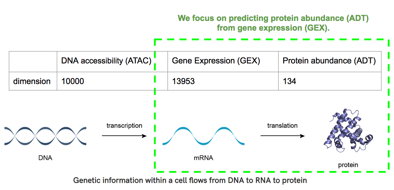
Thanks to single-cell technology, we can measure multiple modalities within the same single cell such as DNA accessibility (ATAC), mRNA gene expression (GEX), and protein abundance (ADT). Figure 1 shows that these modalities are intrinsically linked. Only accessible DNA can produce mRNA, which in turn is used as a template to produce protein.

The problem of modality prediction arises naturally where it is desirable to predict one modality from another. In the 2021 NeurIPS challenge, we were asked to predict the flow of information from ATAC to GEX and from GEX to ADT.

If a machine learning model can make good predictions, it must have learned intricate states of the cell and it could provide a deeper insight into cellular biology. Extending our understanding of these regulatory processes is also transformative for drug target discovery.

The modality prediction is a multi-output regression problem, and it presents unique challenges:

• High cardinality. For example, GEX and ADT information are described in vectors of length 13953 and 134, respectively.
• Strong bias. The data is collected from 10 diverse donors and four sites. Training and test data come from different sites. Both donor and site strongly influence the distribution of the data.
• Sparsity, redundancy, and non-linearity. The modality data is sparse, and the columns are highly correlated.

In this post, we focus on the task of GEX to ADT predictions to demonstrate the efficiency of a single-GPU solution. Our methods can be extended to other single-cell modality prediction tasks with larger data size and higher cardinality using multi-node multi-GPU architectures.

Using TSVD and KRR algorithms for multi-target regression

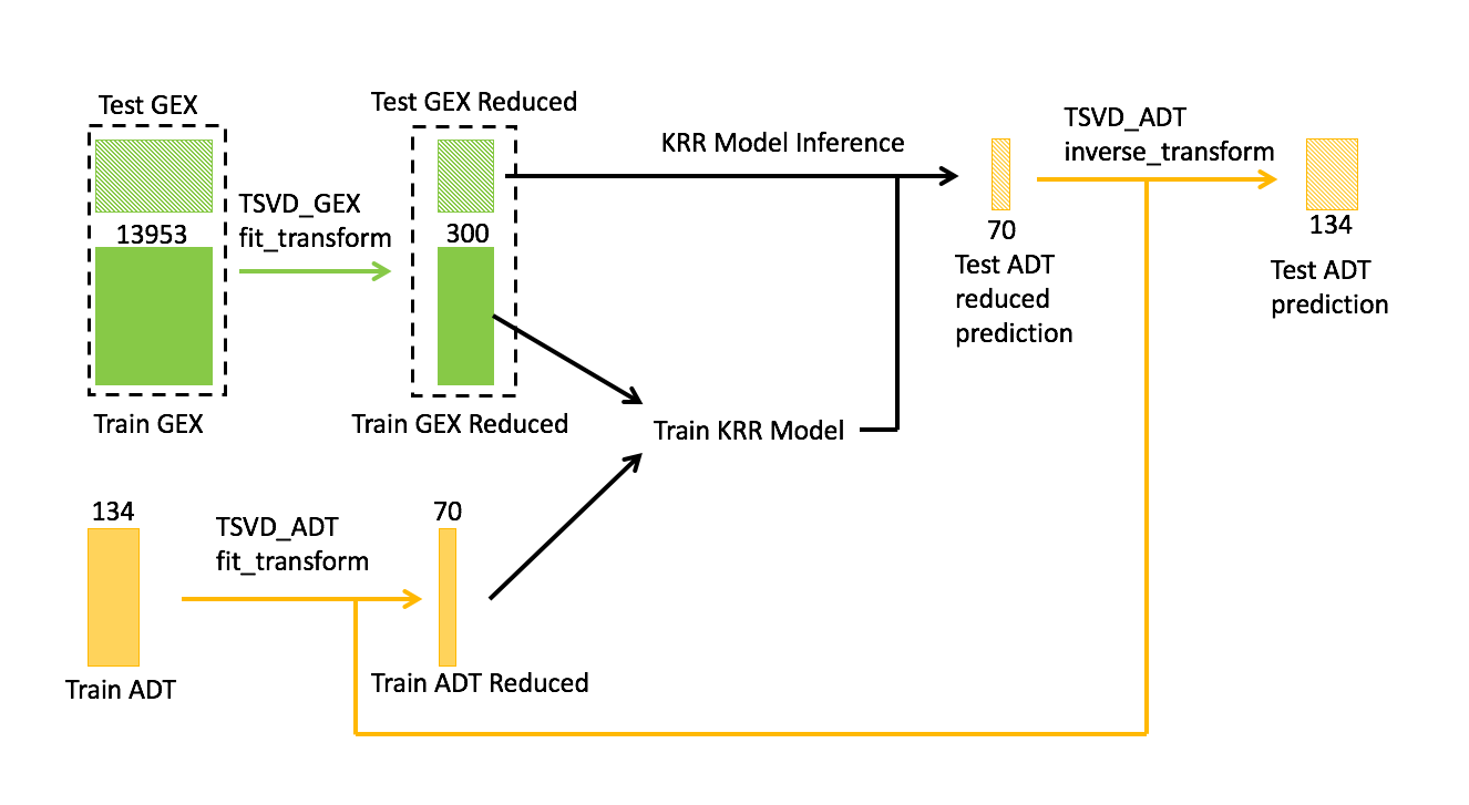
As our baseline, we used the first-place solution of the NeurIPS Modality Prediction Challenge “GEX to ADT” from Kaiwen Deng of University of Michigan. The workflow of the core model is shown in Figure 2. The training data includes both GEX and ADT information while the test data only has GEX information.

The task is to predict the ADT of the test data given its GEX. To address the sparsity and redundancy of the data, we applied truncated singular value decomposition (TSVD) to reduce the dimension of both GEX and ADT.

In particular, two TSVD models fit GEX and ADT separately:

• For GEX, TSVD fits the concatenated data of both training and testing.
• For ADT, TSVD only fits the training data.

In Deng’s solution, dimensionality is reduced aggressively from 13953 to 300 for GEX and from 134 to 70 for ADT.

The number of principal components 300 and 70 are hyperparameters of the model, which are obtained through cross-validation and tuning. The reduced version of GEX and ADT of training data are then fed into KRR with the RBF kernel. Matching Deng’s approach, at inference time, we used the trained KRR model to perform the following tasks:

• Predict the reduced version of ADT of the test data.
• Apply the inverse transform of TSVD.
• Recover the ADT prediction of the test data.

Generally, TSVD is the most popular choice to perform dimension reduction for sparse data, typically used during feature engineering. In this case, TSVD is used to reduce the dimension of both the features (GEX) and the targets (ADT). Dimension reduction of the targets makes it much easier for the downstream multi-output regression model because the TSVD outputs are more independent across the columns.

KRR is chosen as the multi-output regression model. Compared to SVM, KRR computes all the columns of the output concurrently while SVM predicts one column at a time so KRR can learn the nonlinearity like SVM but be much faster.

Implementing a GPU-accelerated solution with cuML

cuML is one of the RAPIDS libraries. It contains a suite of GPU-accelerated machine learning algorithms that provide many highly optimized models, including both TSVD and KRR. You can quickly adapt the baseline model from a scikit-learn implementation to a cuML implementation.

In the following code example, we only needed to change six lines of code and three of them are imports. For simplicity, many preprocessing and utility codes are omitted.

from sklearn.decomposition import TruncatedSVD
from sklearn.gaussian_process.kernels import RBF
from sklearn.kernel_ridge import KernelRidge

tsvd_gex = TruncatedSVD(n_components=300)
tsvd_adt = TruncatedSVD(n_components=70)

gex_train_test = tsvd_gex.fit_transform(gex_train_test)
gex_train, gex_test = split(get_train_test)
adt_train = tsvd_adt.fit_transform(adt_train)
adt_comp = tsvd_adt.components_

y_pred = 0
for seed in seeds:
    gex_tr,_,adt_tr,_=train_test_split(gex_train, 
                                       adt_train,
                                       train_size=0.5, 
                                       random_state=seed)
    kernel = RBF(length_scale = scale)
    krr = KernelRidge(alpha=alpha, kernel=kernel)
    krr.fit(gex_tr, adt_tr)
    y_pred += (krr.predict(gex_test) @ adt_comp)
y_pred /= len(seeds)

from cuml.decomposition import TruncatedSVD
from cuml.kernel_ridge import KernelRidge
import gc

tsvd_gex = TruncatedSVD(n_components=300)
tsvd_adt = TruncatedSVD(n_components=70)

gex_train_test = tsvd_gex.fit_transform(gex_train_test)
gex_train, gex_test = split(get_train_test)
adt_train = tsvd_adt.fit_transform(adt_train)
adt_comp = tsvd_adt.components_.to_output('cupy')

y_pred = 0
for seed in seeds:
    gex_tr,_,adt_tr,_=train_test_split(gex_train, 
                                       adt_train,
                                       train_size=0.5, 
                                       random_state=seed)
    krr = KernelRidge(alpha=alpha,kernel='rbf')
    krr.fit(gex_tr, adt_tr)
    gc.collect()
    y_pred += (krr.predict(gex_test) @ adt_comp)
y_pred /= len(seeds)

The syntax of cuML kernels is slightly different from scikit-learn. Instead of creating a standalone kernel object, we specified the kernel type in the KernelRidge’s constructor. This is because the Gaussian process is not supported by cuML yet.

Another difference is that explicit garbage collection is needed for the current version cuML implementations. Some form of reference cycles are created in this particular loop and objects are not freed automatically without garbage collection. For more information, see the complete notebooks in the /daxiongshu/rapids_nips_blog GitHub repo.

Results

We compared the cuML implementation of TSVD+KRR against the CPU baseline and other top solutions in the challenge. The GPU solutions run on a single V100 GPU and the CPU solutions run on dual 20-core Intel Xeon CPUs. The metric for the competition is root mean square error (RMSE).

We found that the cuML implementation of TSVD+KRR is 103x faster than the CPU baseline with a slight degradation of the score due to the randomness in the pipeline. However, the score is still better than any other models in the competition.

We also compared our solution with two deep learning models:

• Fourth place solution Multilayer Perceptron (MLP)
• Second place solution Graph Neural Network (GNN)

Both deep learning models are implemented in PyTorch and run on a single V100 GPU. Both deep learning models have many layers with millions of parameters to train and hence are prone to overfitting for this dataset. In comparison, TSVD+KRR only has to train less than 30K parameters. Figure 4 shows that the cuML TSVD+KRR model is both faster and more accurate than the deep learning models, thanks to its simplicity.

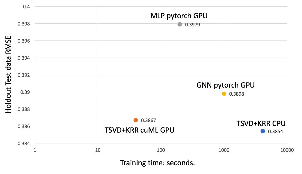
Figure 5 shows a detailed speedup analysis, where we present timings for the two stages of the algorithm: TSVD and KRR. cuML TSVD and KRR are 15x and 103x faster than the CPU baseline, respectively.

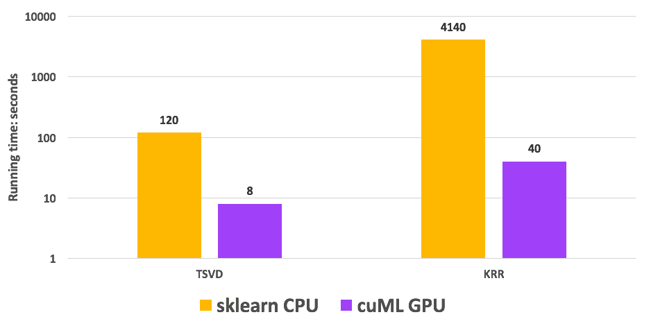
Figure 5. Run time comparison

Conclusion

Due to its lightning speed and user-friendly API, RAPIDS cuML is incredibly useful for accelerating the analysis of the single-cell data. With a few minor code changes, you can boost your existing scikit-learn workflows.

In addition, when dealing with single-cell modality prediction, we recommend starting with cuML TSVD to reduce the dimension of data and KRR for the downstream tasks to achieve the best speedup.

Try out this RAPIDS cuML implementation with the code on the /daxiongshu/rapids_nips_blog GitHub repo.