Quantum dynamics describes how complex quantum systems evolve in time and interact with their surroundings. Simulating quantum dynamics is extremely difficult yet critical for understanding and predicting the fundamental properties of materials.
This is of particular importance in the development of quantum processing units (QPUs), where quantum dynamics simulations enable QPU developers to understand the physics of and improve their hardware.
Quantum dynamics simulations differ from the prevalent circuit simulations used to study how future quantum algorithms will run. Circuit simulations model the evolution of qubits under the application of discrete quantum logical gates. This simplified view idealizes how qubits interact with their surroundings, precluding the consideration of real-world noise and other factors.
In contrast, quantum dynamics simulations comprehensively represent how quantum systems evolve in time, revealing fundamental limits on the speed and accuracy of quantum processes.
To make a classical analogy, the logic of a classical computer can be modeled using binary logic (AND, OR, XOR) applied to transistors, represented abstractly as 0s and 1s. However, to design faster and higher-performing transistors, electrical engineers run complex models that fully simulate device physics, including fluctuations in voltage, capacitance, and current.
The same logic follows for designing better qubits and QPUs, with analog dynamics simulations fully capturing the physics of a QPU. This is the quantum equivalent of modeling the physics of transistors.
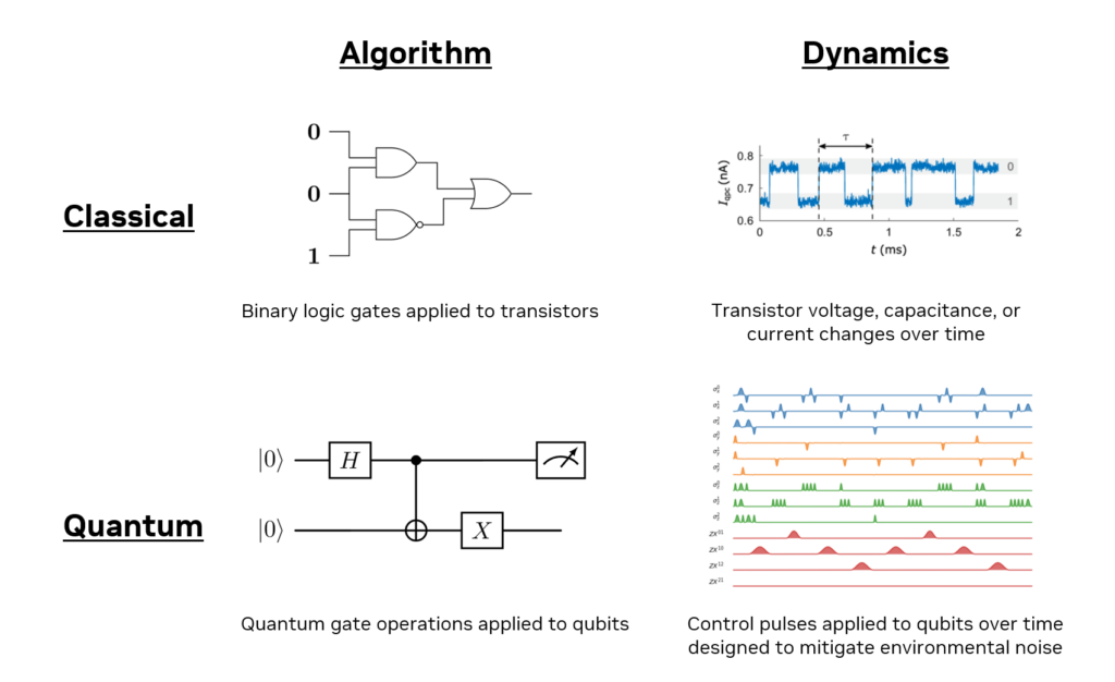
Dynamics simulations are computationally demanding. As the sizes of QPUs increase, they only become feasible when accelerated by GPU supercomputing.
NVIDIA now offers tools that bring GPU-accelerated quantum dynamics simulations within the reach of all QPU researchers and developers:
- The new dynamics APIs built into the NVIDIA CUDA-Q platform can be used in conjunction with several prepackaged solvers (tools to solve the underlying differential equations).
- Researchers can tap directly into the powerful code driving CUDA-Q dynamics calculations, and use the low-level NVIDIA cuQuantum SDK library to develop quantum dynamics simulators around their own custom solvers.
This post explores how Google has been using this CUDA-Q functionality to simulate components of their QPUs. It also benchmarks the performance of both CUDA-Q dynamics and cuQuantum-driven simulations and provides a walkthrough for getting started with CUDA-Q dynamics calculations.
Accelerating Google’s quantum computing R&D
Google, in collaboration with NVIDIA, is accelerating their solvers to run simulations to guide their QPU development. Accurate simulation can serve as a digital representation of a QPU and can often circumvent the need for expensive or impractical experiments in the design process. Google has developed its own solvers by drawing on the dynamics API provided by the lower-level cuQuantum library.
Google and NVIDIA have already used dynamics simulations to explore two initial systems:
- A Heisenberg model spin-chain with the Google QPU operating in analog mode. Accurate results from simulations of this system provide the ground truth for benchmarking Google’s QPU and identifying promising applications for running when it is in analog mode.
- A transmon qubit coupled to a resonator and Purcell filter, which is a key subsystem that bottlenecks the speed at which superconducting qubits can be measured.
A 40-qubit spin-chain simulation was completed using the multi-GPU, multinode capabilities provided by the cuQuantum dynamics APIs (Figure 2). The simulation used 1,024 NVIDIA H100 GPUs in the NVIDIA Eos AI supercomputer. This is the largest exact dynamical simulation of a QPU ever performed to date and opens the door for Google to explore previously intractable systems.
In Figure 2, the bright blue and yellow points indicate measurements applied to individual qubits with increasing frequency, creating a measurement-induced phase transition and the resulting localized quantum states.
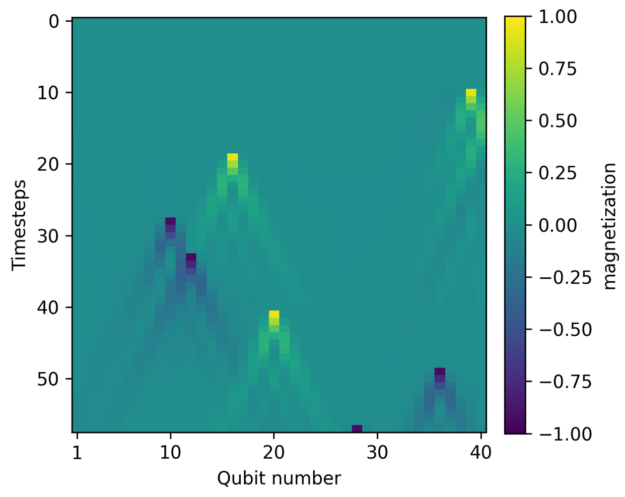
The Google results show how multinode, multi-GPU capabilities can bring simulations to bear on problem sizes previously beyond the reach of researchers. The software also exhibits impressive strong scaling as more GPUs are added.
Figure 3 shows the master equation evaluation runtimes for simulating a transmon qubit with up to 64 levels, coupled to a resonator with up to 256 levels, and a Purcell filter with four levels (64, 256, 4) while increasing the number of GPUs. Assuming a workflow of 100 time steps (four actions per time step with RK4 integration, for a total of 400 operator actions), the time to solution decreases from over 12 days with Qiskit Dynamics, run on a dual-socket Intel Xeon 8480CL, to 2 minutes with cuQuantum using eight GPUs for the largest system benchmarked.
The results from this simulation provide direct benefit to Google’s hardware development cycle. By simulating larger unit cells of the device faster, Google can better identify promising designs before fabrication, saving significant time and resources.

Accelerating quantum dynamics with CUDA-Q
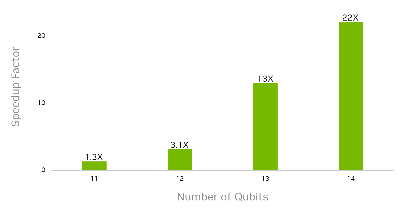
CUDA-Q also provides the additional capability to fully simulate an entire workflow with its own in-built solvers, including the solution of the Lindblad master equation with a time integrator. Single GPU benchmarks of an N qubit spin chain were performed using CUDA-Q–provided solvers with up to 14 noisy qubits on a single NVIDIA H100 GPU.
Results are compared against the best runtime from two leading CPU simulators (run on Intel Xeon Platinum 8480CL) and one leading GPU simulator (Figure 4). Only one of the CPU simulators has sufficient memory to simulate systems of more than 12 qubits. For the 14 qubit simulation, CUDA-Q is nearly 22x faster while the other CPU simulator slows down exponentially as the number of qubits is increased.
Build your own accelerated simulations
You can easily prepare your own GPU-accelerated simulations using the quantum dynamics capabilities of NVIDIA CUDA-Q. This section outlines an example that uses CUDA-Q to simulate a transmon qubit coupled to a resonator based on the paper, Charge Insensitive Qubit Design Derived from the Cooper Pair Box.
The objective of this simulation is to understand how particle number and quadrature of the system evolve over time. The quadrature is a key observable used to understand the transmon qubit measurement process. The following steps show how simple it is to use CUDA-Q to run a quantum dynamics simulation for this use case.
First, CUDA-Q is imported along with the necessary auxiliary package and CUDA-Q is set to the dynamics target.
import cudaq
from cudaq import operators, spin, Schedule, ScipyZvodeIntegrator
from cudaq.operator import coherent_state
import numpy as np
import cupy as cp

cudaq.set_target("dynamics")
Next, the simulation parameters used in the paper are prepared.
# Number of cavity photons
N = 20

# System dimensions: transmon + cavity
dimensions = {0: 2, 1: N}

# System parameters
# Unit: GHz
omega_01 = 3.0 * 2 * np.pi  # transmon qubit frequency
omega_r = 2.0 * 2 * np.pi   # resonator frequency

# Dispersive shift
chi_01 = 0.025 * 2 * np.pi
chi_12 = 0.0
CUDA-Q is then used to define common operators such as creation, annihilation, number, and Pauli operators. The code also sets aliases for the cavity and transmon operators to be used in this simulation.
# Alias for commonly used operators
# Cavity operators
a = operators.annihilate(1)
a_dag = operators.create(1)
nc = operators.number(1)
xc = operators.annihilate(1) + operators.create(1)

# Transmon operators
sz = spin.z(0)
sx = spin.x(0)
nq = operators.number(0)
xq = operators.annihilate(0) + operators.create(0)
Having specified operators and parameters, the effective Hamiltonian of the system, \(\hat{H}_{\mathrm{eff}} = \frac{\hbar\omega’_{01}}{2}\hat{\sigma}_z + (\hbar\omega’_r +\hbar\chi\hat{\sigma}_z)\hat{a}^\dagger\hat{a}\), is defined. For more information about the derivation of this Hamiltonian, see section 3.8 of Charge Insensitive Qubit Design Derived from the Cooper Pair Box.
omega_01_prime = omega_01 + chi_01
omega_r_prime = omega_r - chi_12 / 2.0
chi = chi_01 - chi_12 / 2.0
hamiltonian = 0.5 * omega_01_prime * sz + (omega_r_prime + chi * sz) * a_dag * a
The initial states of the transmon and the cavity also need to be prepared. For this example, choose to prepare both in a superposition state.
# Transmon in a superposition state
transmon_state = cp.array([1. / np.sqrt(2.), 1. / np.sqrt(2.)],
                          dtype=cp.complex128)

# Cavity in a superposition state
cavity_state = coherent_state(N, 2.0)
psi0 = cudaq.State.from_data(cp.kron(transmon_state, cavity_state))
Finally, the schedule is specified. This sets the integration time steps for the simulation and any other parameters to capture.
steps = np.linspace(0, 250, 1000)
schedule = Schedule(steps, ["time"])
This provides all the prerequisites needed to run the simulation using the evolve function, which takes the Hamiltonian, system dimensions, schedule, initial states, and observables as inputs. An integrator for performing the numerical time integration can also be specified. This example uses one from the Python scientific computation library, SciPy:
evolution_result = cudaq.evolve(hamiltonian,
                          dimensions,
                          schedule,
                          psi0,
                          observables=[nc, nq, xc, xq],
                          collapse_operators=[],
                          store_intermediate_results=True,
                          integrator=ScipyZvodeIntegrator())
After the simulation is complete, expectation values can be extracted to retrieve quantities like cavity photon number and quadrature. The observables list defined in the previous code example determines which observables are computed and how they are indexed.
get_result = lambda idx, res: [
    exp_vals[idx].expectation() for exp_vals in res.expectation_values()
]
count_results = [
    get_result(0, evolution_result),
    get_result(1, evolution_result)
]

quadrature_results = [
    get_result(2, evolution_result),
    get_result(3, evolution_result)
]
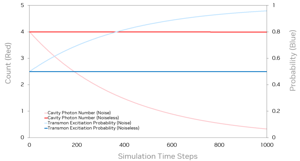
The noisy results can be generated by including collapse operators in the simulation earlier, which decay both the transmon and the cavity. The procedure is the same, but in this case, the collapse operators—0.1*a and 0.1*spin.minus(0)—are included in the previously empty collapse_operators list and the evolve function is called again. To see the full code to produce the results with and without noise, see the /NVIDIA/cuda-quantum GitHub repo.
Figure 5 shows the results with and without noise for the cavity photon number and the transmission excitation probability. The introduction of noise results in more realistic behavior where the cavity photon number decreases over time. The quadrature results also obtained from this simulation can be used to better understand how the transmon qubit interacts with the resonator during measurement.
For more information about how to simulate other systems and to learn more about the other features that can be used in dynamical simulations, see the CUDA-Q dynamics node in the GitHub repo. This includes an example of preparing a simulation that can run directly on a QuEra analog quantum processor, using the same APIs and requiring minimal code changes.
Get started
The new CUDA-Q and cuQuantum dynamics capabilities enable researchers to run quantum dynamics simulations at speeds and scales that were simply not possible in the past. As QPU builders scale their hardware into the regime of early quantum error correction, a tool with this capability becomes essential.
Download CUDA-Q to start experimenting with dynamic simulations. You can immediately run code, taking advantage of its built-in solvers. To see a few dynamics example notebooks, see /NVIDIA/cuda-quantum on GitHub.
If you want to build your own custom quantum dynamics solvers, download cuQuantum to accelerate them by multiple orders of magnitude.
Learn more about NVIDIA quantum computing.

