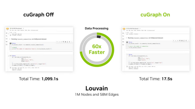
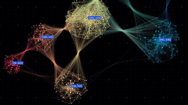
NetworkX is a popular, easy-to-use Python library for graph analytics. However, its performance and scalability may be unsatisfactory for medium-to-large-sized networks, which can significantly hinder user productivity.
NVIDIA and ArangoDB have collectively addressed these performance and scaling issues with a solution that requires zero code changes to NetworkX. This solution integrates three main components:
- The NetworkX API
- Graph acceleration using RAPIDS cuGraph
- Production-ready analytics at scale in ArangoDB
In this post, I discuss how this makes life easier for NetworkX users, show you an example implementation, and explain how to get started with early access.
Easy graph analytics with NetworkX
NetworkX is widely used by data scientists, students, and many others for graph analytics. It is open-source, well-documented, and supports plenty of algorithms with a simple API.
That said, one known limitation is its performance for medium-to-large graphs, which significantly hampers its usefulness for production applications.
Accelerating graph analytics with cuGraph
The RAPIDS cuGraph graph analytics acceleration library bridges the gap between NetworkX and GPU-based graph analytics:
- Graph creation and manipulation: Create and manipulate graphs using NetworkX, with data seamlessly passed to cuGraph for accelerated processing on large graphs.
- Fast graph algorithms: Real-time analytics using the power of NVIDIA GPUs.
- Data interoperability: Support for data in NetworkX graph objects and other formats, enabling simple data exchange between machine learning, ETL tasks, and graph analytics.
The best part? You get the benefits of GPU acceleration without changing your code. Just install the nx-cugraph library and specify the cuGraph backend. For more information about installation and performance benchmarks, see Accelerating NetworkX on NVIDIA GPUs for High Performance Graph Analytics.
In short, for varying sizes of k from 10–1000, GPUs speed up a single run of betweenness centrality by 11–600x.
Production-ready graph analytics with ArangoDB
NetworkX users have typically had to undertake a complex set of methods for persisting graph data:
- Manual data exports to flat files
- Relational databases
- Ad-hoc solutions, such as using in-memory storage
Each of these methods has a unique set of challenges and forces you to spend time and effort managing and manipulating graph data rather than focusing on analysis and data science tasks.
ArangoDB’s data persistence layer makes it easier for one or more users to perform graph operations on any network too large to fit in memory. By integrating ArangoDB as the persistent data layer, you will see several potential benefits:
- Scalability: Graph data can scale horizontally, not just vertically, across multiple nodes, handling large datasets.
- Performance: Fast read and write operations for real-time analysis and manipulation of graph data.
- Flexibility: Support for all popular data models: graph, document, full-text search, key/value, and geospatial, all in a single, fully integrated platform. Multi-tenancy is also supported.
Figure 1 shows how integrating ArangoDB into the workflow of NetworkX users transforms the way graph data is stored and accessed. By providing this new persistence layer, ArangoDB enables data scientists to focus on what they do best, not data manipulation and other minutia.

Data persistence enables users to take advantage of work done by other team members. Data does not have to be loaded from the source and compiled into a graph for each user. Instead, they can load the graph from the database.
The results of graph algorithms can also be stored and retrieved rather than run again by every single user. Ultimately, this saves users time and money.
GPU-accelerated analytics with cuGraph and ArangoDB
Large datasets take a long time to analyze in NetworkX. That’s why ArangoDB uses RAPIDS cuGraph to analyze graph data, especially when data grows large enough that performance slows down.
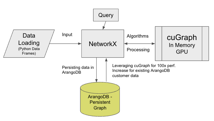
There are several benefits to scaling ArangoDB with GPUs through a NetworkX interface. First, data extraction from ArangoDB is much faster with a GPU compared to a CPU. That is because ArangoDB optimizes its data extraction tools to uniquely cater to cuGraph data structures, namely the coordinate list (COO) graph format.
Second, you can analyze large graph data through your laptop or another client. NetworkX acts as a client API library for graph algorithms that require more memory than the client could provide.
Finally, no code changes are necessary. cuGraph supports zero code changes for NetworkX users so you can use tools that are already familiar to you.
Example implementation
Thanks to the capabilities of the NetworkX backend-to-backend interface, nx-arangodb graphs can use the GPU capabilities of nx-cugraph, as long as an NVIDIA GPU is available on the machine. In other words, the choice to run CPU or GPU algorithms through NetworkX remains when using nx-arangodb.
The following sections show how to create and persist a graph in ArangoDB using NetworkX and the nx-arangodb library:
- Downloading the data
- Creating the NetworkX graph
- Running a cuGraph algorithm without ArangoDB
- Persisting the NetworkX graph to ArangoDB
- Instantiating the NetworkX-ArangoDB graph
- Running a cuGraph algorithm with ArangoDB
Test environment
For this post, I used an Intel Xeon CPU with 13 GB of system RAM and compared it against an NVIDIA A100 GPU with 84 GB of system RAM and 40 GB of GPU RAM. I worked with CUDA 12.2.
The Stanford Network Analysis Platform (SNAP) Citation Patents dataset is a citation graph of patents granted between 1975 and 1999, totaling 3.7M nodes and 16.5M edges. The code examples rely on the betweenness centrality graph algorithm to help you find which patents are more central than others and get an idea of their relative importance.
For this post, I used an ArangoDB instance provisioned through the ArangoGraph Managed Service, which enabled me to persist any created graphs for future sessions. It is running as Enterprise Edition 3.11.8 as a sharded database with six nodes, each with 32 GB of memory.
Step 0: Downloading the data
First, download the Citation Patents dataset and write it to a text file.
# Median Time: 10 seconds

import gzip
import shutil
import requests

url = 'https://snap.stanford.edu/data/cit-Patents.txt.gz'
name = 'cit-Patents.txt'

# Download gz
response = requests.get(url, stream=True)
response.raise_for_status()

# Stream gz data & write to text file
with response.raw as r, gzip.open(r, 'rb') as f_in, open(name, 'wb') as f_out:
    shutil.copyfileobj(f_in, f_out)
Step 1: Creating the NetworkX graph
Next, instantiate the NetworkX graph using a pandas edge list.
# Median Time: 90 seconds

import pandas as pd
import networkx as nx

# Read into Pandas
pandas_edgelist = pd.read_csv(
    "cit-Patents.txt",
    skiprows=4,
    delimiter="\t",
    names=["src", "dst"],
    dtype={"src": "int32", "dst": "int32"},
)

# Create NetworkX Graph from Edgelist
G_nx = nx.from_pandas_edgelist(
    pandas_edgelist, source="src", target="dst", create_using=nx.DiGraph
)
Step 2: Running a cuGraph algorithm without ArangoDB
A NetworkX algorithm can be invoked with backend set to cugraph. This uses the GPU-accelerated algorithm implementation of nx-cugraph with zero code changes.
# Median Time: 5 seconds

result = nx.betweenness_centrality(G_nx, k=10, backend="cugraph")
Alternately, set the NETWORKX_AUTOMATIC_BACKENDS environment variable to specify cugraph as the selected NetworkX backend instead of specifying the backend parameter.
Step 3: Persisting the NetworkX graph to ArangoDB
At this point, you can choose to persist the local NetworkX graph into ArangoDB. Assuming that you have an ArangoDB instance running at the DATABASE_HOST provided, you can load the graph by instantiating a nxadb.DiGraph object, and using the incoming_graph_data parameter along with a specific name.
# Median Time: 3 Minutes

import os
import nx_arangodb as nxadb

os.environ["DATABASE_HOST"] = "https://123.arangodb.cloud:8529"
os.environ["DATABASE_USERNAME"] = "root"
os.environ["DATABASE_PASSWORD"] = "password"
os.environ["DATABASE_NAME"] = "myDB"

# Load the DiGraph into ArangoDB
G_nxadb = nxadb.DiGraph(
    name="cit_patents",
    incoming_graph_data=G_nx,
    write_batch_size=50000
)
Now, assume that a new Python session has been created. It is up to you whether to create the new session on the same machine or a different machine. This can be useful when you are working with a teammate for collaborative development.
Step 4: Instantiating the NetworkX-ArangoDB Graph
Re-connecting to the persisted graph can be done by specifying the connection credentials using environment variables and re-instantiating nxadb.DiGraph. Optional read_batch_size and read_parallelism parameters are provided for optimizing data read.
Graph instantiation does not pull the graph into memory but establishes the remote connection to the persisted graph.
# Median Time: 0 seconds

import nx_arangodb as nxadb

os.environ["DATABASE_HOST"] = "https://123.arangodb.cloud:8529"
os.environ["DATABASE_USERNAME"] = "root"
os.environ["DATABASE_PASSWORD"] = "password"
os.environ["DATABASE_NAME"] = "myDB"

# Connect to the persisted Graph in ArangoDB
# This doesn't pull the graph; You're just establishing a remote connection.
G_nxadb = nxadb.DiGraph(
    name="cit_patents",
    read_parallelism=15,
    read_batch_size=3000000
)
Step 5: Running a cuGraph algorithm with ArangoDB
With the use of a GPU, you can rely on the same algorithm to fetch the GPU representation of the ArangoDB graph, which has a significantly smaller memory footprint than that of the CPU representation. After the ArangoDB graph has been pulled, it is cached as a NetworkX-cuGraph graph, which enables you to run more algorithms without needing to pull it again unless the user specifically requests to do so.
# Option 1: Explicit Graph Creation

from nx_arangodb.convert import nxadb_to_nxcg

# Pull the graph from ArangoDB and cache it
# Median Time: 30 seconds
G_nxcg = nxadb_to_nxcg(G_nxadb)

# Median Time: 5 seconds
result = nx.betweenness_centrality(G_nxcg, k=10)
# Option 2 (recommended): On-demand Graph Creation
# This pulls the graph from ArangoDB on the first algorithm call & caches it

# Median Time: 35 seconds
result = nx.betweenness_centrality(G_nxadb, k=10)
Verdict: Data persisted in ArangoDB
Given the new ability to persist NetworkX graphs in ArangoDB, you can load new sessions 3x faster than without having a database involved.
| Description | Steps | Time (sec) |
| Without data persisted in ArangoDB | 0-2 | 105 |
| Data persisted in ArangoDB | 5 | 35 |
| Speedup | 3X |
Running multiple sessions on the data or requiring multiple people to analyze the same data without ArangoDB would require the inconvenience of starting from scratch. Having a persistence layer facilitates this workflow. It makes the combination of cuGraph and ArangoDB a key strategy for working with large graphs in NetworkX.
Step 6: Using CRUD functionality with NetworkX-ArangoDB
More functionality is available with NetworkX-ArangoDB should you choose to use it for CRUD functionality. NetworkX-ArangoDB puts a strong emphasis on zero-code change, implying that the CRUD interface for NetworkX-ArangoDB Graphs is identical to that of NetworkX graphs.
Persisting to ArangoDB also enables you to take advantage of ArangoDB’s multi-model query language; the Arango Query Language (AQL). This is a unified query language to perform graph traversals, full-text search, document retrieval, and key-value lookups on one platform.
import nx_arangodb as nxadb

G_nxadb = nxadb.DiGraph(name="cit_patents") # Connect to ArangoDB

assert G_nxadb.number_of_nodes() == G_nx.number_of_nodes()
assert G_nxadb.number_of_edges() == G_nx.number_of_edges()
assert len(G_nxadb[5526234]) == len(G_nx[5526234])

G_nxadb.nodes[1]["foo"] = "bar"
del G_nxadb.nodes[1]["foo"]

G_nxadb[5526234][4872081]["object"] = {"foo": "bar"}
G_nxadb[5526234][4872081]["object"]["foo"] = "bar!"
del G_nxadb[5526234][4872081]["object"]

G_nxadb.add_edge("A", "B", bar="foo")
G_nxadb["A"]["B"]["bar"] = "foo!"
del G_nxadb.nodes["A"]
del G_nxadb.nodes["B"]
Conclusion
Combining the NetworkX Graph API with persistence in ArangoDB and fast processing with cuGraph gives you a production-quality workbench for building models and processes. This technical integration between ArangoDB and NVIDIA represents a major evolution in graph database analytics.
By persisting graph data in ArangoDB, you will find that you can avoid the complexities and inefficiencies typical of manual data exports or using in-memory storage. To be precise, in-memory storage, while fast in some cases, is not ideal for large graphs because of memory constraints and the high risk of data loss during system crashes and other unplanned downtime.
For NetworkX users, ArangoDB offers an ideal and easy-to-implement transparent persistence layer, transforming how graph data is stored and accessed. You can now run large-scale graph analytics without leaving the familiarity of NetworkX. Existing ArangoDB customers will also see the benefits of advanced graph analytics and accelerated performance of NetworkX backed by cuGraph.
For more information about the full potential of this powerful integration and to get early access, see Introducing The ArangoDB NetworkX Persistence Layer.

