Sparse tensors are vectors, matrices, and higher-dimensional generalizations with many zeros. They are crucial in various fields such as scientific computing, signal processing, and deep learning due to their efficiency in storage, computation, and power. Despite their benefits, handling sparse tensors manually or through existing libraries is often cumbersome, error-prone, nonportable, and does not scale with the combinatorial explosion of sparsity patterns, data types, operations, and targets.
Research largely focuses on sparse storage formats—data structures that compactly store nonzeros and allow efficient operations that avoid redundancies such as x+0=x and x*0=0. This enables scaling to larger sizes or solving same sizes with fewer resources. No single sparse format is optimal; the best choice depends on the nonzero distribution, operations, and target architecture.
The Universal Sparse Tensor (UST) decouples a tensor’s sparsity from its memory storage representation. The UST uses a domain-specific language (DSL) to describe how a tensor should be represented in memory. Developers focus on the sparsity of a tensor only. Compile-time or runtime inspection of the chosen format for the operands in sparsity-agnostic polymorphic operations eventually decides between dispatching to an optimized handwritten library or otherwise with automatic sparse code generation when no such solution exists. The UST has its roots in sparse compiler technology; see, for example, Compiler Support for Sparse Matrix Computations, Sparse Tensor Algebra Compilation and Compiler Support for Sparse Tensor Computations in MLIR.
This post focuses on how developers can use the UST to define common but also less common sparse storage formats, each tailored to specific properties of the sparse tensors that occur in their application. Operability with, for example, SciPy, CuPy, and PyTorch sparse tensors maps common formats like COO, CSR, and DIA to the corresponding DSL of the UST. However, developers can also define their own novel sparsity format by means of the DSL. Combined with dispatch or code generation, this allows the design of novel sparse formats without explicit coding, as will be shown in future posts.
The tensor format DSL
The tensor format DSL maps tensor dimensions (logical tensor indices) to storage levels (physical memory indices) using an invertible function that defines how each level should be stored. It consists of:
1. An ordered sequence of dimension specifications, such as (i, j), each of which includes a dimension-expression to provide a named reference to each dimension.
2. An ordered sequence of level specifications, such as (i : dense, j : compressed), each of which includes a level expression, which defines what is stored in each level, and a required level type, which defines how the level is stored, including:
- A collection of level properties, such as unique and ordered
- A required level format, such as:
- dense: Meaning that the underlying storage only involves indexing similar to a dense array
- compressed: Meaning that at that level, a positions array defines the locations of a stored level and a coordinates array is used to store the indices within each stored level
- singleton: A compressed variant where each coordinate directly belongs to the parent at the previous level
- range: A dense dense variant where coordinate values are based on a compression at a prior level
The positions and coordinates arrays are stored as jagged (variable-sized) arrays, first indexed by level, namely pos[l], and then by content, where the positions use the convention that two consecutive elements define a half-open interval from pos[l][i] up to pos[l][i+1]. Where unused, jagged arrays are left empty. At the end of all levels, a single values array contains the linearized numerical values of all stored elements. What makes the UST universal is that the DSL above can be easily extended to include even more storage formats.
UST examples
The UST examples in this section show that the different possibilities of storing dense and sparse tensors grows rapidly with the dimensionality.
Scalars
A scalar is a 0-dimensional (0D) tensor, so there are no dimensions and thus no levels. As such, the values array in the UST storage consists of a single “dense” element that contains the scalar value (Figure 1).
() -> () # scalar

Vectors
A vector is a 1-dimensional (1D) tensor that can be interpreted visually as either a row or column vector. A sample sparse row vector is shown in Figure 2.

Two common ways of storing a vector dense or compressed are shown below:
(i) -> (i : dense)         # dense vector
(i) -> (i : compressed)    # sparse vector
Figure 3 shows the UST storage of the sample vector using these two formats. Dense storage uses zero padding to get filled levels in the values array. The positions and coordinates arrays are unused. Sparse storage uses the positions array to define the half-open interval [0,5), where there are coordinates and values of each element.

It’s also possible to map a single dimension to two levels to obtain blocked vector storage. An example that defines block size 4 is shown below, which essentially maps a 1D dimension space, named i, into a 2D level space (i/4,i%4).
(i) -> (i / 4 : compressed, i % 4 : dense) # blocked vector
Figure 4 shows UST storage of the sample vector. Zero padding is used to get filled blocks. The positions array in the first level denotes that two dense blocks are stored using [0,2). Arrays at the second level are unused. As shown in red, the element with, for example, index 8 and value -1 is mapped to inter-block level index 2 and intra-block level index 0.

Matrices
Sparse matrix storage (2D) has been studied extensively and many widely adopted sparse storage formats exist, each with a unique name. The flexibility of the UST is able to define most of them, thereby unifying many variations under a single umbrella.
If using just the level formats dense/compressed combined with index permutations, the tensor format DSL of a d-dimensional tensor already gives rise to 2d✕d! different combinations. For d=2, this evaluates to eight different matrix formats.
(i, j) -> (i : dense, j : dense)              # Dense (row-major)
(i, j) -> (j : dense, i : dense)              # Dense (col-major)
(i, j) -> (i : dense, j : compressed)         # CSR
(i, j) -> (j : dense, i : compressed)         # CSC
(i, j) -> (i : compressed, j : compressed)    # DCSR
(i, j) -> (j : compressed, i : compressed)    # DCSC
(i, j) -> (i : compressed, j : row)           # CROW (less common)
(i, j) -> (j : compressed, i : row)           # CCOL (less common)
Dense storage using either row-major or column-major order is straightforward. Figure 5 shows the CSR format of a sample 4×5 matrix with six nonzero elements. Because level 0 is dense, arrays pos[0], crd[0] are unused. Instead, the i-index is used as an index into level 1 to find compressed storage of that row.
There, two consecutive positions pos[1][i] and pos[1][i+1] define a half-open interval of locations into the coordinates array used to reconstruct the j-index of every stored value. (Given this concise way of encoding, the size of the pos array must always be one more than the actual dimension size.) This is the last level, so the actual numerical values can be found at the same positions in the values array.

Looking at other level types, the COO format is expressed using the DSL shown below. Here the compressed level uses the nonunique property to denote that the same index can appear multiple times. The second level uses the singleton level format to denote that no positions array is required since each index is associated directly with its parent.
(i, j) -> (i : compressed(nonunique), j : singleton) # COO
Storing the hyper sparse matrix in Figure 6 in COO yields the given UST format. Coloring is used to denote the storage relation of element a22=3. Like previous formats, the UST COO format also corresponds one-to-one with the COO format found in the literature, except for the somewhat unusual initial positions array to define the number of stored elements.

The range level format can be combined with level expressions involving add/sub to define diagonal and antidiagonal storage of elements. Here, there is a choice to use either the row index or column index into the actually stored dense diagonal, giving rise to four variants.
(i, j) -> (j-i : compressed, i : range)    # DIA-I
(i, j) -> (j-i : compressed, j : range)    # DIA-J
(i, j) -> (i+j : compressed, i : range)    # ANTI-DIA-I
(i, j) -> (i+j : compressed, j : range)    # ANTI-DIA-J
The difference between using either a row or column index only becomes apparent for nonsquare matrices. The sample 5×7 matrix in Figure 7 shows both the DIA-I and DIA-J formats in Figures 8 and 9. Coloring is used to relate stored diagonals back to the matrix diagonals. The format uses zero padding inside and outside the range to reach completely filled levels (where, unlike inside padding, outside padding does not correspond to elements within the original matrix index space).

Figure 8 shows the DIA-I format.

Figure 9 is the DIA-J format for the same matrix. Selecting the index of the larger dimension results in more zero padding, so that the DIA-I format would be preferred in this case.

Many more storage variations can be obtained with blocking, where 2D indices map into either 3D levels (into strips) or 4D levels (into blocks). For the latter, even though the literature typically only mentions BSR and BSC to define row-major or column-major order between the blocks, the tensor format DSL of the UST more precisely also distinguishes between row-major and column-major format within each stored block, giving rise to the following four variants for 2×3 blocks.
(i, j) -> (i / 2 : dense, j / 3 : compressed,
           i % 2 : dense, j % 3 : dense)     # BSR-Row(2,3)
(i, j) -> (i / 2 : dense, j / 3 : compressed,
           j % 3 : dense, i % 2 : dense)     # BSR-Col(2,3)
(i, j) -> (j / 3 : dense, i / 2 : compressed,
           i % 2 : dense, j % 3 : dense)     # BSC-Row(2,3)
(i, j) -> (j / 3 : dense, i / 2 : compressed,
           j % 3 : dense, i % 2 : dense)     # BSC-Col(2,3)
The 4×9 matrix in Figure 10 is used to illustrate block storage. Block B11 is colored red to highlight where it actually resides. For example, entry a25=16 can be found mapping dimension indices (2,5) to the level indices (1, 1, 0, 2): block B11 indexed by (0,2). Because compressed row-major storage of blocks makes this the fourth stored block (after B00, B02, and B10), while dense row-major storage within the block makes this the third entry there, eventually this translates to the element at index 20 of the values array.

These examples should provide an impression of the expressiveness of the tensor format DSL in describing sparse matrix storage formats. The following sections explore higher dimensions.
Tensors
As previously discussed, just using dense/compressed level types with index permutations in the UST tensor format DSL gives rise to 2d✕d! different ways of storing tensors. For d=3, d=4, d=5, and d=6 this yields 48, 384, 3,840, and 46,080 combinations, respectively—simply too many to list here. Adding the other level types increases this number even further.
To provide a few examples of storing 3D tensors: the dimension permutations of the UST allows for six different direct ways of storing 3D dense tensors, varying from the classic row-major to column-major and everything swiveling in between. Storing a 3D tensor with all levels compressed gives rise to the CSF (compressed sparse fiber) format.
(i, j, k) -> (i : compressed, j : compressed, k : compressed) # CSF
Consider the 3D 4x3x5 tensor in Figure 11, which is visualized on paper by showing the underlying 2D 3×5 matrices in a row for i=0, i=1, i=2 (empty), and i=3.

Representing this tensor using the CSF format as UST yields the storage shown in Figure 12. The coloring indicates how the stored element a320=8 is found. Such a format is suitable for very sparse tensors where the nonzeros are uniformly distributed over all dimensions.

A 3D tensor can be thought of as a batched set of matrices, a popular concept in DL. Placing the batch dimension at different levels can sometimes have interesting consequences on the uniformity of sparsity within the batch. Consider the 3D 4x5x5 tensor of Figure 13, visualized as a batch of 5×5 matrices.

Given the diagonal nature within the matrices, it makes sense to store this tensor as a batched DIA format. The most natural way is keeping the batch dimensional variable i as the outermost dense level, followed by diagonal storage of the matrices.
(i, j, k) -> (i : dense, k-j : compressed, j : range) # batched DIA-I
This nonuniform batched DIAG-I storage is shown in Figure 14, where each batch can have its own diagonal structure. Color relates one particular diagonal back to its stored location. Zero padding occurs, both inside and outside the stored diagonals, in order to get completely filled dense levels. The coordinates array denotes where diagonals reside (for example, at -1, 0, +1 for the first matrix, and -1 and 0 for the last matrix).

It’s possible to make a subtle change in the tensor format DSL by permuting the batch variable below the diagonal computation:
(i, j, k) -> (k-j : compressed, i : dense, j : range)  # uniform
                                                       # batched CSR
Now metadata for the diagonals is stored only once, but at the expense of forcing a uniform diagonal nonzero pattern on all matrices in the batching, which may require additional zero padding, as can be seen in Figure 15.

Learn more
This post has illustrated the breadth of tensor storage formats encompassed by the UST. Stay tuned for the integration of the UST with polymorphic operations that dispatch to optimized libraries or automatically generated code. This approach establishes a clean, easy-to-use, and scalable sparse ecosystem, facilitating the introduction of novel storage schemes without explicit coding.
Want to learn more? Sign up for the NVIDIA GTC 2026 session, Accelerating GPU Scientific Computing with nvmath-python for a demo on UST and exciting product updates.

