
This post was originally published on the RAPIDS AI blog.
In this post we take a look at how to use cuDF, the RAPIDS dataframe library, to do some of the preprocessing steps required to get the mortgage data in a format that PyTorch can process so that we can explore the performance of deep learning on tabular data and compare it to the xgboost method.

Using the GPU for ETL and preprocessing of deep learning workflows
Deep learning is, however, making inroads into tabular data problems. Recent Kaggle competition winners of the Santander, Porto Seguro, and Taxi Trajectory competitions used deep learning as a significant part of their solution, and the Rossman store sales (#3 solution) and Petfinder competitions (#6 and #9 solution) both had interesting architectures and methodologies that used DNNs to achieve top ten rankings. The Petfinder solutions are of particular interest because they combine tabular, image and text data in a single model. Many companies have come forward stating that they use deep learning in these or similar contexts, including Google, Pinterest, Twitter, Instacart, and Youtube. Deep learning library fast.ai has even added support for tabular data directly into the library in the form of categorical embeddings and a range of preprocessing options required for tabular data.
Please check out the accompanying notebook in the RAPIDS.AI repo for the implementation details. The notebook and experiments were developed and run by Christopher Green and we’re grateful for his work.
Establishing a baseline
As our starting point we’ll take the original mortgage notebook from the RAPIDS repo. Feature engineering is identical in order to prevent performance improvements unrelated to deep learning.
Here, when we say performance, we’re talking about how well the algorithm is able to classify loans, which we’ll measure as the Area Under the Precision Recall Curve, or PR-AUC for short. We chose PR-AUC over cross entropy, accuracy and ROC-AUC because we think it provides a better representation of the performance of the algorithm. Lowest cross entropy loss often doesn’t correspond to the most accurate model when examining the model’s ability to predict whether a loan will go delinquent. On the other hand, using accuracy as the only metric hides precision/recall tradeoffs necessary when evaluating a model in the real world. Finally, ROC-AUC is less able to distinguish between model performance when there is a class imbalance, which we see in the mortgage dataset.
We use a time-based split of the data, creating validation and test sets such that they occur after the training data in order to prevent data leakage. Since we’re predicting 12-month loan delinquency we need to ensure that the validation and test data start at least 12 months after the latest date in the training dataset. Similarly, we establish a test set from a later time window than the validation set to ensure that we don’t overfit the hyperparameters.
Because of the size of the dataset (1.75 billion rows!) and the nature of xgboost on GPU which requires the entire training dataset to be in memory, we are only able to train on 17% with a single DGX-1 server, which has eight Tesla-V100 32GB GPUs. A single V100 can handle ~2% of the dataset. If you were to try to run this on commodity hardware like a GTX 1080-ti you’d be limited to ~0.7% of the dataset. By taking advantage of the GPU’s massive parallelism along with recent optimizations, we’re able to train the multi-gpu xgboost model in an astonishing 60 seconds. The full run time including ETL and preprocessing is 178 seconds. Scaling resources to a six-node cluster allows training across the entire dataset with similar timing, but that isn’t the focus of this post.
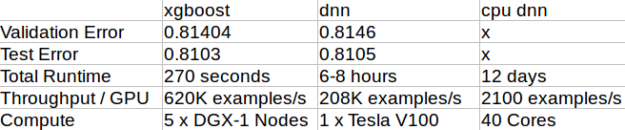
After running a hyperparameter search we achieved a best PR-AUC of 0.814104 on the validation set, which corresponds to 0.8103 on the test set. This is the benchmark we try to reach or beat using a deep learning model.
Deep learning specific data transforms
There are many ways of encoding tabular data into a format that a deep neural network (DNN) can understand. One common approach is to one-hot encode categorical variables and to normalize continuous variables before feeding them directly into the first feed-forward layer. However, in our experience, this is not very effective. In our own previous testing across multiple datasets, DNNs that use one-hot encoding wasn’t competitive with gradient boosting methods.
More recently, categorical embeddings — sometimes referred to as entity embeddings — have become popular for dealing with categorical variables. Categorical embeddings assign a learnable feature vector, or embedding, to each category, generally with a size correlated with the number of unique values in that category. Each unique category value has its own associated vector, allowing for a rich representation of the data where the values are represented as multiple floating-point values, rather than a single binary. The categorical embedding outputs and normalized continuous variables are then concatenated together as the input to the model.
Bag-of-features type approaches have also been used, where all of the features are embedded in the same size embedding and the input to the model is composed of the sum of its feature embeddings. This technique is modelled after bag-of-words techniques from natural language processing, the most famous of which is word2vec.
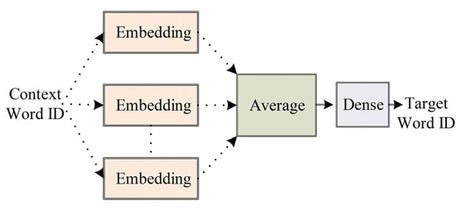
This first RAPIDS+Deep Learning notebook uses the bag-of-features approach, mapping all categorical and continuous variables into a single latent space, and uses an EmbeddingBag layer to take the average of all of the feature embeddings. These aggregated features are then fed into a sequence of four linear layers of width 600. Future posts will explore a wider range of options, and introduce some new ways of processing tabular data and new architectures for tabular data, an area of research that we are actively exploring.
Continuous input variables
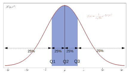
To map continuous variables to an embedding space they must be discretized. We’ve added functionality to the cuDF Series to map a continuous input into buckets based on quantiles which split a distribution into equal parts. In this context, we’re converting continuous variables to categoricals in order to take advantage of the power of embeddings. For our quantization in this notebook we use a quantile of 20 regions, each with 5% of the input distribution. A quantile dividing into four regions is shown below for a normal distribution to demonstrate how the split is applied when the data isn’t uniform.
Sharing an embedding space
Because we’re mapping all of our categorical and continuous variables into the same embedding space when using the bag of features model, we also need to make sure that the same value in different categories is handled correctly and isn’t mapped to the same id. To ensure this happens we hash the name of the input column with the value to create a unique id representing the value in that specific column. These are then mapped to an embedding bag so that all embeddings for an entry can be looked up and combined in a single pass. Hashing of a series was also added to cuDF to make this step easy.
Implementation details
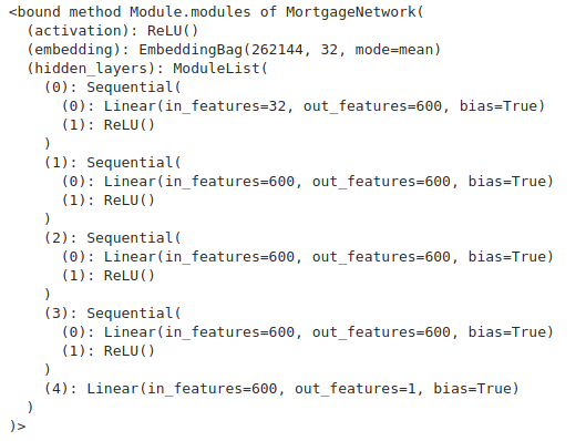
Our final model is an EmbeddingBag layer followed by several feedforward layers as seen below. We perform a small hyperparameter search exploring learning rate [log_uniform(1e-4..1e-2)], weight decay [uniform(1e-6..1e-4)], batch size [512, 1024, 4096, 8192], embedding size [8, 16, 24, 32, 64], and activation type [relu, selu]. 200 different combinations were randomly sampled and evaluated using the validation set.
Results and key takeaways
The best performing DNN model on the validation set (PR-AUC of 0.8146) is able to achieve a PR-AUC of 0.8105 on our test set, slightly better than that of the xgboost model. The final hyperparameters are as follows: [lr = 2.005e-3, wd = 8e-6, batch size = 8192, embedding size = 32]
Key takeaways:
- Even with a simple architecture, we’re able to achieve similar performance to xgboost with deep learning.
- The deep learning model processes 208K examples/s during training, taking 6–8 hours including preprocessing and ETL on a single V100. That’s much slower than the 4.95M examples/s xgboost model that ran in 60 seconds on a DGX-1 server; but it is roughly comparable considering it equates to 620K examples/s per GPU. In future posts we’ll explore mixed precision, multi-gpu and other techniques to speed up the training of our DNN model. Our CPU benchmark processes only 2100 examples/s on a 40 core machine, which clearly demonstrates why we’re doing deep learning on GPUs. The CPU system would take over 12 days to complete a single run!
- While slower, using data loaders, we are able to train across the entire dataset using a single GPU, which is an advantage in many applications. Currently this process involves batchwise transfer of data between the CPU and GPU. In future posts we’ll be exploring in-GPU-memory data loaders to dramatically speed up training.
This first foray into deep learning for RAPIDS.AI is a significant step, demonstrating that we can achieve similar performance to xgboost with DNNS with a reasonably simple model and motivating further exploration.
Next steps
In future posts we’ll undertake the following explorations.
- Simplify preprocessing of tabular data on GPUs and explore more direct ETL pipelines for getting data directly into a format that PyTorch and other deep learning frameworks can work with.
- Introduce some of the trappings of modern deep learning like dropout, batchnorm, learning rate schedules, concatenated embeddings, etc., and explore different architectures for tabular deep learning.
- Evaluate the performance of deep learning for tabular data on a wider range of datasets.
- Explore multi-GPU and multi-node scaling of DNN models.
In the meantime, please take a deeper look at the notebook, adapt it to your favourite dataset, and let us know your experience.
Get in touch and shape the future of RAPIDS
RAPIDS relies on your feedback to make it a great platform for data science on GPUs. We’re excited to blur the lines between data analytics and deep learning. RAPIDS is committed to providing a first-class user experience, so thank you for being a part of this community.
You can install the latest release with Conda or use the container found on NVIDIA GPU Cloud or Docker Hub. Let us know what you think via GitHub stars and issues.
