Gone are the days of using a single GPU to train a deep learning model. With computationally intensive algorithms such as semantic segmentation, a single GPU can take days to optimize a model. But multi-GPU hardware is expensive, you say. Not any longer; NVIDIA multi-GPU hardware on cloud instances like the AWS P3 allow you to pay for only what you use. Cloud instances allow you to take advantage of the latest generation of hardware with support for Tensor Cores, enabling significant performance boots with modest investments. You may have heard that setting up a cloud instance is difficult, but NVIDIA NGC makes life much easier. NGC is the hub of GPU-optimized software for deep learning, machine learning, and HPC. NGC takes care of all the plumbing so developers and data scientists can focus on generating actionable insights.
This post walks through the easiest path to speeding up semantic segmentation by using NVIDIA GPUs on a cloud instance with the MATLAB container for deep learning available from NGC. First, we will explain semantic segmentation. Next we will show performance results for a semantic segmentation model trained in MATLAB on two different P3 instances using the MATLAB R2018b container available from NGC . Finally, we’ll cover a few tricks in MATLAB that make it easy to perform deep learning and help manage memory use.
What is Semantic Segmentation?
The semantic segmentation algorithm for deep learning assigns a label or category to every pixel in an image. This dense approach to recognition provides critical capabilities compared to traditional bounding-box approaches in some applications. In automated driving, it’s the difference between a generalized area labeled “road” and an exact, pixel-level determination of the drivable surface of the road. In medical imaging, it means the difference between labeling a rectangular region as a “cancer cell” and knowing the exact shape and size of the cell.
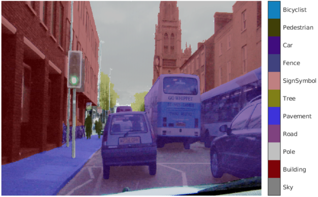
We tested semantic segmentation using MATLAB to train a SegNet model, which has an encoder-decoder architecture with four encoder layers and four decoder layers. The dataset associated with this model is the CamVid dataset, a driving dataset with each pixel labeled with a semantic class (e.g. sky, road, vehicle, etc.). Unlike the original paper, we used stochastic gradient descent for training and pre-initialized the layers and weights from a pretrained VGG-16 model.
Performance Testing Using MATLAB on P3 Instances with NVIDIA GPUs
While semantic segmentation can be effective, it comes at a significant computational and memory cost. We ran our tests using AWS P3 instances with the MATLAB container available from NGC . Use of the container requires an AWS account and a valid MATLAB license. You can obtain a free trial MATLAB license for cloud use. Mathworks makes available directions on how to set up the MATLAB container on AWS.
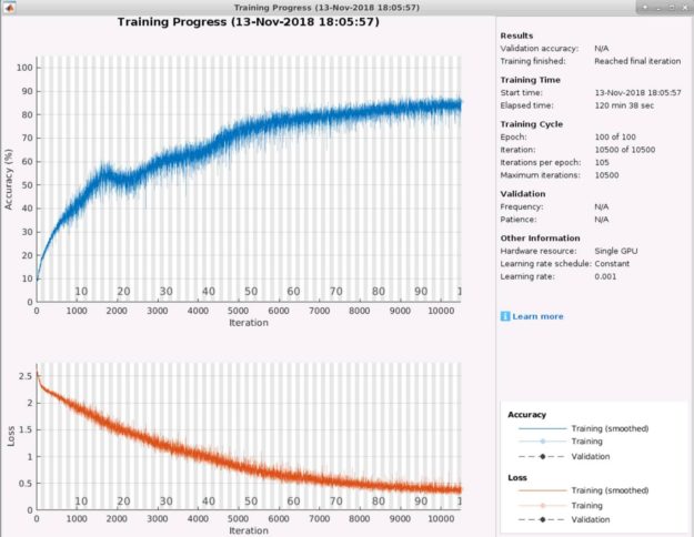
The original SegNet implementation in 2015 took about a week to run on the single Tesla K40 used by the authors, as mentioned in the original paper. Below is a plot of the semantic segmentation network training process in MATLAB using a single V100 NVIDIA GPU on a p3.2xlarge instance. Figure 2 shows it took about 121 minutes, which is much faster than in the original paper.
Next, we performed the same test using the eight V100 NVIDIA GPUs available on a p3.16xlarge instance. The only change required in the MATLAB code: setting the training option parameter ExecutionEnvironment to multi-gpu. Figure 3 illustrates a training plot showing that the process now took 37 minutes, 3.25x faster than using the p3.2xlarge instance.
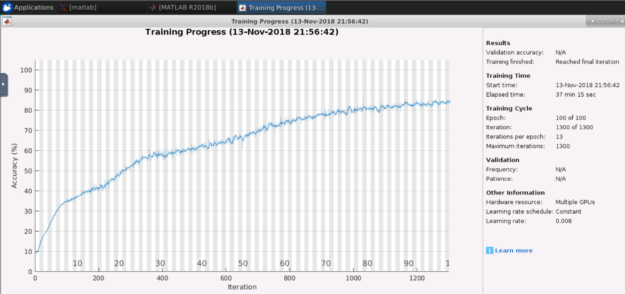
This 3.25x improvement in performance shows the power of the latest NVIDIA multi-GPU hardware with Tensor Cores, bringing what originally took “about a week” down to 37 minutes. I bet the SegNet authors wish they had this hardware when they were developing their algorithm!
Making Deep Learning Easier with MATLAB
Now let’s dive into why you should use MATLAB for developing deep learning algorithms such as semantic segmentation. MATLAB includes many useful tools and commands to make it easier to perform deep learning. One of the most useful MATLAB commands is imageDatastore, which allows you to efficiently manage a large collection of images. The command creates a database that allows working with the entire dataset as a single object. The MiniBatchSize parameter is particularly critical for semantic segmentation, determining how many images are used in each iteration. The default value of 256 consumes too much memory for semantic segmentation, so we set the value to 4.
Data augmentation, as presented in the function imageDataAugmenter, represents another powerful deep learning capability in MATLAB. Data augmentation extends datasets by providing more examples to the network using translations, rotations, reflections, scaling, cropping, and more. This helps improve model accuracy. This uses data augmentation of random left/right reflections and X/Y translations of +/- 10 pixels. This data augmentation is combined into a pixelLabelDatastore, so that the operations occur at the time of each iteration and avoids unnecessary copies of the dataset.
How We Performed Semantic Segmentation in MATLAB
This section covers key parts of the code we used for the test above. The complete MATLAB code used in this test is available here. The single line at the end is where the training occurs.
The following code downloads the dataset and unzips it on your local machine.
imageURL = 'http://web4.cs.ucl.ac.uk/staff/g.brostow/MotionSegRecData/files/701_StillsRaw_full.zip';
labelURL = 'http://web4.cs.ucl.ac.uk/staff/g.brostow/MotionSegRecData/data/LabeledApproved_full.zip';

outputFolder = fullfile(tempdir,'CamVid');

if ~exist(outputFolder, 'dir')

    mkdir(outputFolder)
    labelsZip = fullfile(outputFolder,'labels.zip');
    imagesZip = fullfile(outputFolder,'images.zip');

    disp('Downloading 16 MB CamVid dataset labels...');
    websave(labelsZip, labelURL);
    unzip(labelsZip, fullfile(outputFolder,'labels'));

    disp('Downloading 557 MB CamVid dataset images...');
    websave(imagesZip, imageURL);
    unzip(imagesZip, fullfile(outputFolder,'images'));
end
This code makes a temporary folder to unzip the files on your instance. When using the container, these files will be lost once the container shuts down. If you want to maintain a consistent location for your data, you should change the code to use an S3 bucket or some other permanent location.
The code below shows 11 classes used from the CamVid dataset to train the semantic segmentation network. In the original dataset, there are 32 classes.
imgDir = fullfile(outputFolder,'images','701_StillsRaw_full');
imds = imageDatastore(imgDir);
classes = [
    "Sky"
    "Building"
    "Pole"
    "Road"
    "Pavement"
    "Tree"
    "SignSymbol"
    "Fence"
    "Car"
    "Pedestrian"
    "Bicyclist"
    ];

labelIDs = camvidPixelLabelIDs();
labelDir = fullfile(outputFolder,'labels');
pxds = pixelLabelDatastore(labelDir,classes,labelIDs);
In this next section, we resize the CamVid data to the resolution of the SegNet and partition the dataset into training and testing sets.
imageFolder = fullfile(outputFolder,'imagesResized',filesep);
imds = resizeCamVidImages(imds,imageFolder);
labelFolder = fullfile(outputFolder,'labelsResized',filesep);
pxds = resizeCamVidPixelLabels(pxds,labelFolder);

[imdsTrain,imdsTest,pxdsTrain,pxdsTest] = partitionCamVidData(imds,pxds);
numTrainingImages = numel(imdsTrain.Files)
numTestingImages = numel(imdsTest.Files)
Now let’s create a SegNet network. Start with VGG-16 weights and adjust them to balance the class weights.
imageSize = [360 480 3];
numClasses = numel(classes);
lgraph = segnetLayers(imageSize,numClasses,'vgg16');

imageFreq = tbl.PixelCount ./ tbl.ImagePixelCount;
classWeights = median(imageFreq) ./ imageFreq;
pxLayer = pixelClassificationLayer('Name','labels','ClassNames',tbl.Name,'ClassWeights',classWeights);
lgraph = removeLayers(lgraph,'pixelLabels');
lgraph = addLayers(lgraph, pxLayer);
lgraph = connectLayers(lgraph,'softmax','labels');
Next, select the training options. The MiniBatchSize parameter is particularly critical for semantic segmentation, determining how many images are used in each iteration. The default value of 256 requires too much memory for semantic segmentation, so we set the value to 4. The ExecutionEnvironment option is set to multi-gpu to use multiple V100 NVIDIA GPUs as found on the p3.16xlarge instance. Check out the documentation for more details on the training options.
options = trainingOptions('sgdm', ...
    'Momentum',0.9, ...
    'ExecutionEnvironment','multi-gpu',...
    'InitialLearnRate',1e-3, ...
    'L2Regularization',0.0005, ...
    'MaxEpochs',100, ...
    'MiniBatchSize',4 * gpuDeviceCount, ...
    'Shuffle','every-epoch', ...
    'Plots','training-progress',...
    'VerboseFrequency',2);
Another powerful capability in MATLAB for deep learning is imageDataAugmenter, which provides more examples to the network and helps improve accuracy. This example uses data augmentation of random left/right reflections and X/Y translations of +/- 10 pixels. This is combined into a pixelLabelDatastore, so that the operations occur at the time of each iteration and avoids unnecessary copies of the dataset.
augmenter = imageDataAugmenter('RandXReflection',true,...
    'RandXTranslation',[-10 10],'RandYTranslation',[-10 10]);
pximds = pixelLabelImageDatastore(imdsTrain,pxdsTrain,...
    'DataAugmentation',augmenter);
Now we can start training. This next line of code for training takes about 37 minutes to run on the p3.16xlarge instance. We measure the time spent training in the plot window for keeping track of training progress. Refer back to figures 2 and 3 to see the measured time taken to run this function on p3.2xlarge and p3.16xlarge instances.
[net, info] = trainNetwork(pximds,lgraph,options);
Conclusion
MATLAB makes it easy for engineers to train deep-learning models that can take advantage of NVIDIA GPUs for accelerating the training process. With MATLAB, switching from training on a single GPU machine to a multi-GPU machine takes just a single line of code, shown in the final code snippet above. We showed how you can speed up deep learning applications by training neural networks in the MATLAB Deep Learning Container on the NGC, which is designed to take full advantage of high-performance NVIDIA® GPUs. As a next step, download the code and try it yourself in MATLAB on an AWS P3 instance.

