Today we’re excited to announce the availability of NVIDIA DIGITS 4. DIGITS 4 introduces a new object detection workflow and DetectNet, a new deep neural network for object detection that enables data scientists and researchers to train models that can detect instances of faces, pedestrians, traffic signs, vehicles and other objects in images.
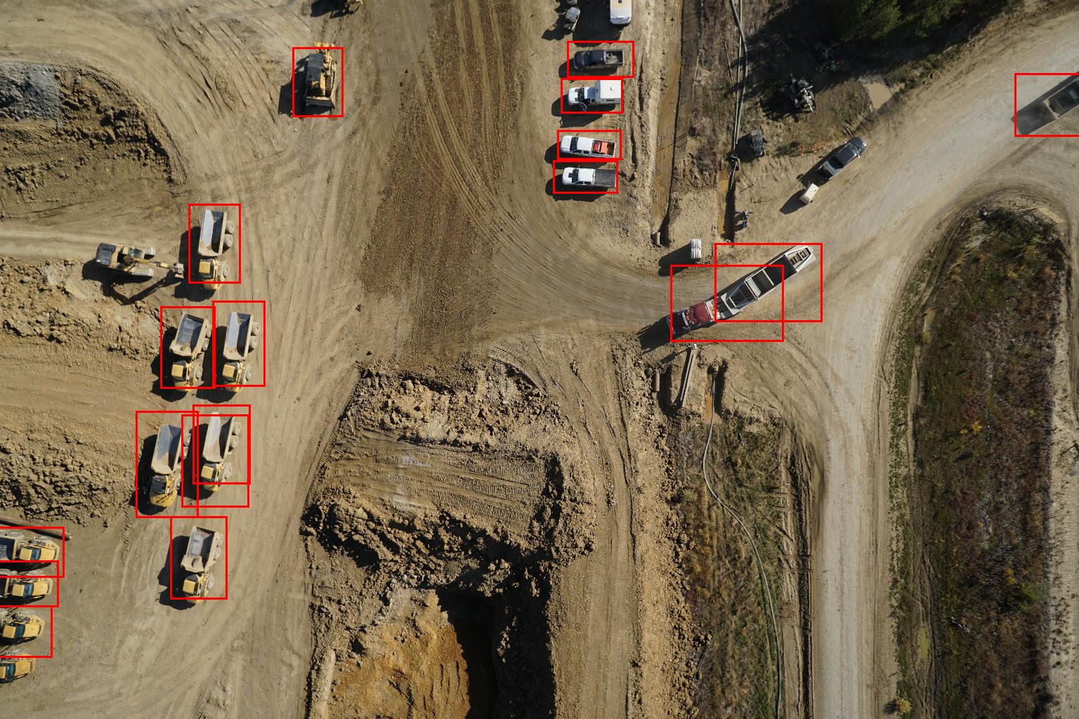
Object detection is one of the most challenging problems in computer vision and is the first step in several computer vision applications. The goal of an object detection system is to detect all instances of objects of a known category in an image. Figure 1 shows the final results of an object detection system trained with DIGITS which can detect vehicles on a construction site. Starting with a successful vehicle detection system like this, you can solve a number of other problems such as recognizing the makes and models of the vehicles, counting and tracking vehicle locations over time, generating natural language descriptions of the images and so on.
In this blog post I’ll introduce object detection and some of its key challenges, and show how you can use DIGITS 4 and DetectNet to train your own object detection system.
Object Detection Challenges
Object detection is a particularly challenging task in computer vision. A good object detection system has to be robust to the presence (or absence) of objects in arbitrary scenes, be invariant to object scale, viewpoint, and orientation, and be able to detect partially occluded objects. Real-world images can contain a few instances of objects or a very large number; this can have an effect on the accuracy and computational efficiency of an object detection system.
Historically, object detection systems depended on feature-based techniques which included creating manually engineered features for each region, and then training of a shallow classifier such as SVM or logistic regression. The proliferation of powerful GPUs and availability of large datasets have made training deep neural networks (DNN) practical for object detection. DNNs address almost all of the aforementioned challenges as they have the capacity to learn more complex representations of objects in images than shallow networks and eliminate the reliance on hand-engineered features.
Most deep-learning-based object detection approaches today repurpose image classifiers by applying them to a sliding window across an input image. Some approaches such as RCNN make region proposals using selective search instead of doing an exhaustive search to save computation, but it still generates over 2000 proposals per image. These approaches are in general very computationally expensive, and do not generate accurate bounding boxes for object detection.
DIGITS 4 includes DetectNet, a new network architecture that simultaneously performs object classification and a regression to estimate object bounding boxes. This means that a single neural network can be trained to predict bounding boxes. The resultant single network offers much higher inference performance than a typical classifier applied as a sliding window detector.
DetectNet is an extension of the popular GoogLeNet network. The extensions are similar to approaches taken in the Yolo and DenseBox papers. If you are interested in the details of the DetectNet architecture, check out the blog post DetectNet: Deep Neural Network for Object Detection in DIGITS.
Object Detection with DIGITS
You can use NVIDIA DIGITS to interactively perform common deep learning tasks such as managing data, defining networks architectures, training multiple models in parallel, and monitoring training performance in real time. If you are new to deep learning with GPUs, DIGITS can get you up and running quickly. For seasoned experts, DIGITS enables you to be more productive by accelerating training on multi-GPU systems, managing multiple training jobs and performing network diagnostics interactively. For more information about how to get started with DIGITS, see our previous blog posts on DIGITS.
Example: Vehicle Detection from Aerial Imagery
For the purposes of this example, I will use an aerial imagery dataset provided by Kespry. Unfortunately, this dataset is not shareable so in order to follow these instruction, I encourage you to use the publically available KITTI dataset or try it with your own dataset. A short walkthrough on how to use the KITTI dataset with DIGITS is also available on the DIGITS GitHub page.
The goal of this example is to detect vehicles in images taken from a commercial drone over a variety of construction sites. This may be be useful for a construction agency for a number of reasons, including counting and tracking the vehicles on the construction site or identifying the types of vehicles on the site such as commercial, delivery or possibly intruders.
Getting started with DIGITS 4
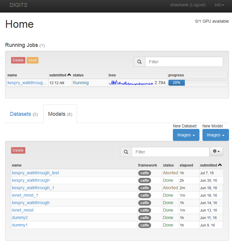
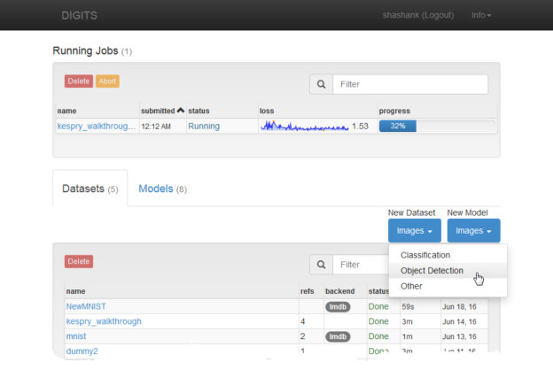
You can download and install DIGITS by following the instructions on the DIGITS home page. After installation is complete, the DIGITS server starts automatically. To start using DIGITS, open up your web browser and navigate to http://localhost/. The DIGITS interface is a web application that you can access from any computer, tablet or mobile device as long as the device has access to the computer running the DIGITS server. Your DIGITS homepage should look like the screenshot in Figure 2.
Loading the Dataset
Supervised learning problems require input/output pairs of data so that the training algorithm can learn how to make predictions on new input data. For example, in image classification the input-output pairs are images and labels for each image.
In the case of object detection with DIGITS 4’s DetectNet, the neural network expects the following input/output data format.
- Input: A folder of images in .png, .jpg, .jpeg, .bmp, .ppm format files.
- Output: A folder containing .txt files where each row contains bounding box coordinates for each occurrence of the object in that image.
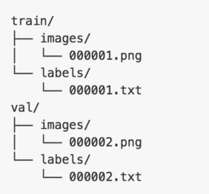
This format is the same as the popular KITTI dataset format. Note that each image (e.g. 000001.jpg) in the image folder must have a corresponding text file in the label folder (e.g. 000001.txt).The image folder and corresponding label folder are contained in the same parent folder. Separate parent folders are used for training and validation datasets. Figure 3 shows a screenshot of the folder structure.
On the DIGITS home page, start by clicking on Images>Object Detection as shown in Figure 4.
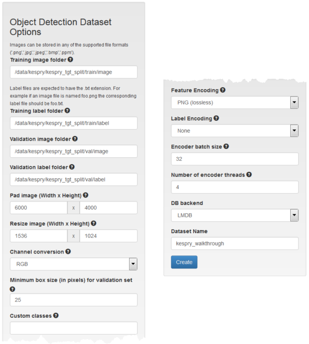
You’ll now be presented with options for creating an object detection dataset.
- Training image folder: The path to the location of the training images.
- Training label folder: The path to the location of the object bounding box text files.
Each instance of the object and its bounding box location should be provided as a dedicated row in the label file. For example, image 68 in Figure 5 has two instances of the object “Car” and these are provided as two separate rows. For a complete list of label parameter descriptions, visit the DIGITS documentation page.

Label files are expected to have the .txt extension. For example if an image file is named foo.png the corresponding label file should be foo.txt.
- Validation image folder: The path to location of the validation images.
- Validation label folder: The path to the location of the object bounding box text files. Use the same format as the training labels.
- Pad image (Width x Height): Pad image with zeros up to specified dimensions, if required.
- Resize image (Width x Height): Resize images to make them compatible with the network architecture. For our example, we specify 1536 x 1024 pixels . This size is used to preserve the original aspect ratio and have sufficient resolution to detect all objects of interest, while minimizing the GPU memory required for training.
Note that in order for DetectNet to successfully detect objects in an image, the object size should be between 50×50 and 400×400 px in the input images.
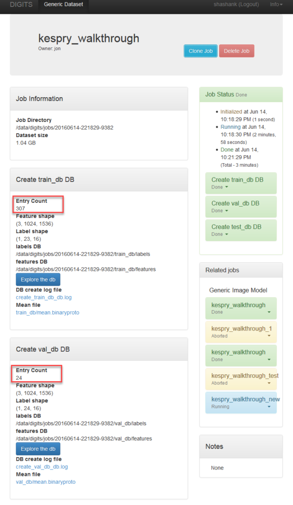
After you have created your dataset you may review the data properties by visiting the dataset page. In Figure 7 you can see that there are 307 training images and 24 validation images.
Model creation
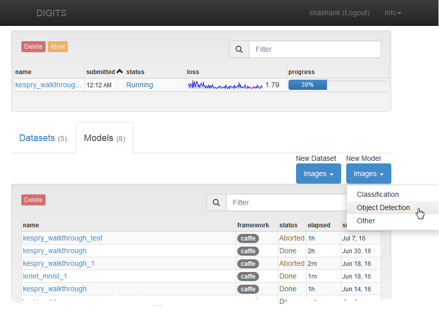
To create your model, navigate to the DIGITS homepage, select the Models tab and click Image > Object Detection as Figure 8 shows.
On the model creation page, you’ll now be presented with options for creating an object detection dataset.
- Select Dataset: Select the dataset you created in the previous section.
- Training epochs: Select 100 training epochs. You can always abort training at any epoch if the desired accuracy is reached.
- Base Learning Rate: Set the base learning rate to
1e-05. You can also specify a learning rate schedule under “advanced learning rate options”. We’ll select “Exponential Decay” for this problem. - Solver Type: Select ADAM (Adaptive Moment Estimation). Use ADAM as an alternative to SGD with Nesterov momentum. You may see faster convergence in some cases.
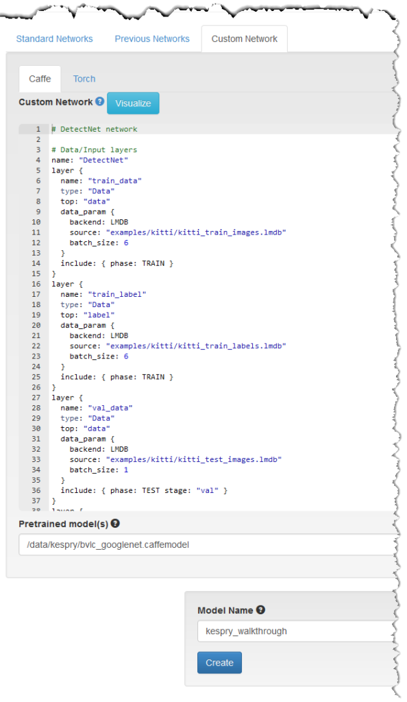
In the network section, select the “Custom Network” tab, and then select the “Caffe” sub-tab. The model description file for DetectNet is in the Caffe examples folder of your DIGITS installation. Navigate to the following location to retrieve the DetectNet model file.
$HOME/caffe/examples/kitti/detectnet_network.prototxt
Simply copy and paste the contents of the ‘detectnet_network.prototxt’ in the custom network window as Figure 9 shows.
Since DetectNet is derived from GoogLeNet I strongly recommend that you use pre-trained weights from an ImageNet-trained GoogLeNet. Under the ‘Pretrained model(s)’ section, provide a path to the pretrained model. You can download a copy of a pre-trained GoogLeNet.caffemodel from the Caffe ModelZoo repository.
DIGITS will automatically initialize the weights of the network with these pretrained values so that it doesn’t have to learn them from scratch. This is an especially good idea if your new training set is not very large—it will save you a lot of training time.
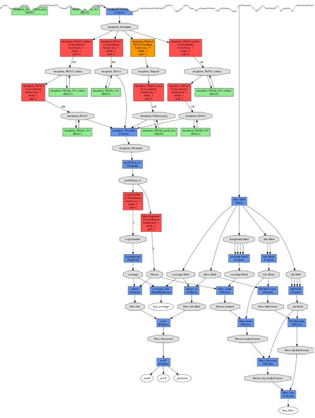
You may click Visualize to review the network topology. As shown in Figure 10. all the layers with red, orange and green are part of the original GoogLeNet architecture. The blue and gray layers at the bottom introduce new loss and clustering function that produce the final set of predicted bounding boxes.
Training DetectNet for Object Detection
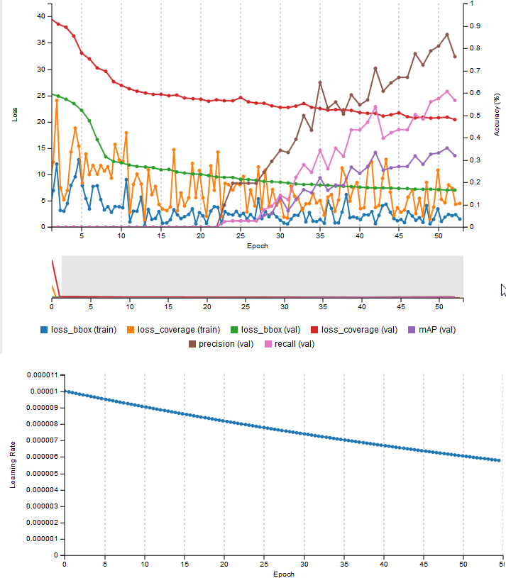
DIGITS starts training the model as soon as you click “create”. Figure 11 shows two graphs that let you monitor training progress. The graph on the top shows curves for the following measures that help you determine how accurate your model is.
- loss_bbox is the mean absolute difference of the true and predicted corners of the bounding box for the object covered by each grid square.
- loss_coverage value of 0 or 1 indicates whether an object is present within the grid square. It is defined as the sum of squares of differences between the true and predicted object coverage across all grid squares in a training data sample.
- Precision is the ratio of the accurately identified objects to the total number of predicted objects (ratio of true positives to true positives plus false positives).
- Recall is the ratio of the accurately identified objects to the total number of actual objects in the images (ratio of true positives to true positives plus false negatives).
- mAP: a simplified mean Average Precision score based on the product of the precision and recall for DetectNet. It’s a good combined measure for how sensitive the network is to objects of interest and how well it avoids false alarms.
The key indicator that the network has learned to detect objects with accurate bounding boxes is a non-zero mAP (mean Average Precision).
Model verification
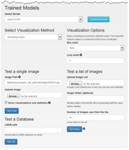
To assess the ability of the model to detect vehicles in the Kespry data and generate accurate bounding boxes you can use the options under Trained Models. The network output is best visualized by drawing bounding rectangles around detected objects.
After navigating to the Trained Models section, you’ll be presented with the following options.
- Select Model: Select the last epoch where the mAP is maximum. If the network starts to overfit at later epochs you may have to choose an earlier epoch based on the validation errors shown in Figure 12.
- Select Visualization Method:
- Bounding Boxes: Displays bounding boxes around detected objects.
- Raw Data: Provides a list of bounding box locations in text.
- Test a single image: Provide a path to the location of a single image that you want to use to test the accuracy of the trained model. Checking the ‘Show visualizations and statistics’ option shows layer-by-layer visualization of the convolutional filters that have been learned, the results of applying these filters to the input data (feature maps), and the heat map of detections and bounding box corner estimates.
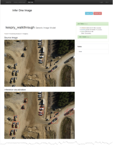
You may also test multiple images at once by specifying the image paths in a text file (one line per image path). Figure 1 Shows the results of performing inference on a single image; as you can see DetectNet is able to successfully detect all instances of cars in the input test image.
Download DIGITS 4 Today
NVIDIA DIGITS makes it easy for scientists, engineers and domain experts who are not deep learning experts to easily perform common deep learning tasks such as managing data, defining network architectures, training models in parallel, and assessing model performance. The new DIGITS 4 object detection workflow and the new DetectNet network let you train custom object detection networks from scratch as I demonstrated in this post.
Get started now by downloading DIGITS 4. DIGITS is an open-source project and free for use.
Already using DIGITS and want to share your experience? Looking for a feature not available in DIGITS? We’d love to hear from you; please leave a comment below.
