
Editor’s note: What happens when a veteran graphics programmer with substantial experience in old-school ray tracing (in other words, offline rendering), gets hold of hardware capable of real-time ray tracing?
I’m finally convinced.
I joined NVIDIA around SIGGRAPH, just as the RTX hardware for ray tracing was announced. I saw the demos, heard the stats, but these didn’t mean a lot to me without hands-on experience.
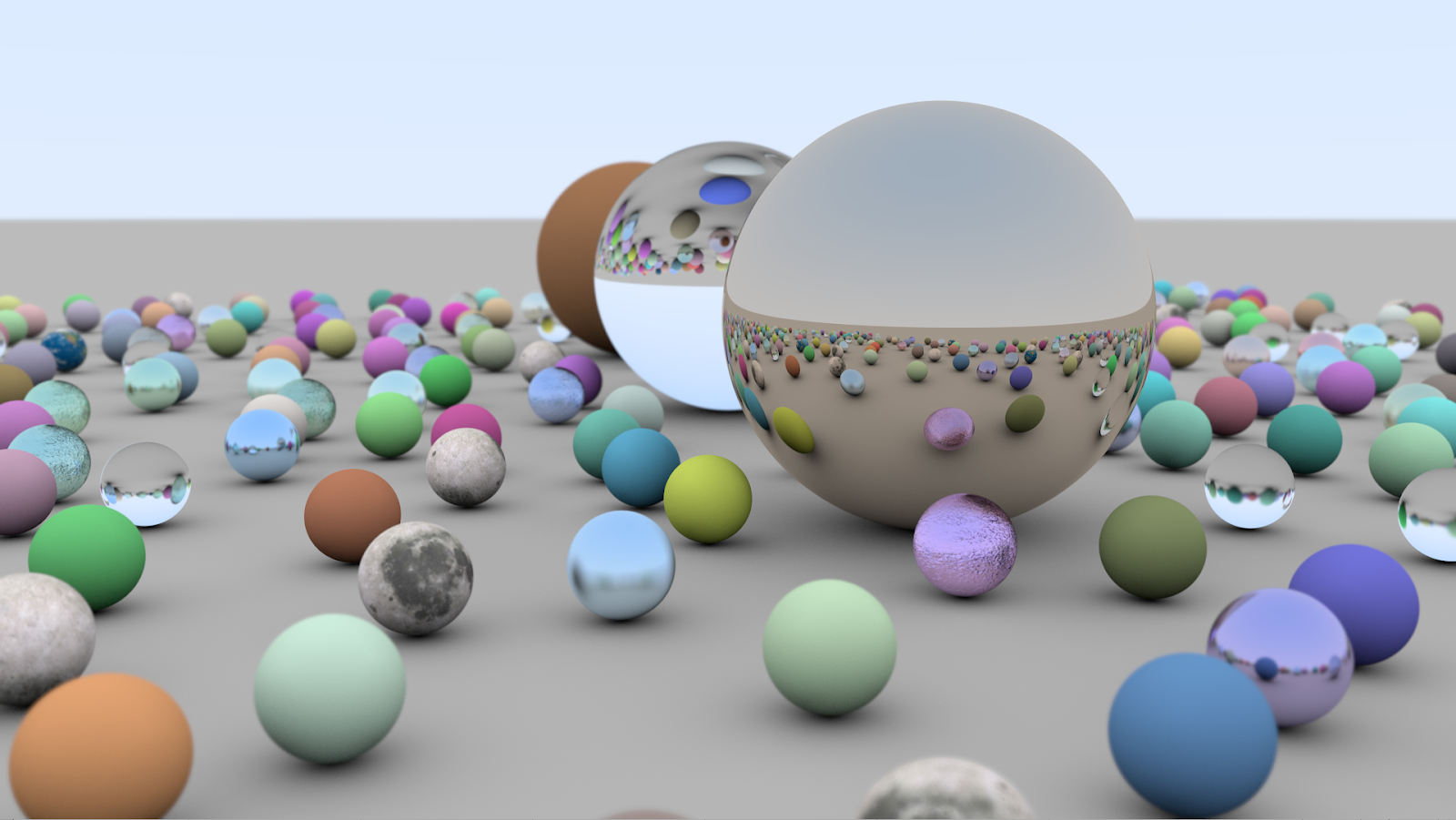
My NVIDIA-issued workstation included an older Titan V card – not a new Turing, but plenty fast, and capable of running DXR ray tracing code. I grabbed Chris Wyman’s tutorials on getting started with ray tracing, then downloaded the free Visual Studio Community edition 2017 and a few other components. The “Ray Tracing in One Weekend” demo seemed particularly appealing, and old-school: all spheres, with classic sharp reflections and refractions, as you see in figure 1. (Pro tip: Pete Shirley’s book explaining this demo, along with his two sequels, are now free – they’re a great way to learn the basics of ray tracing.)
More, More!
The “One Weekend” demo is fine, but the hemispherical light source and lack of denoising makes it noisy when you move through the scene. You can crank up the eye rays per pixel to around 10 and still get about 30 FPS. But, it’s still a bit noisy and, well, it’s “just” 433 spheres.
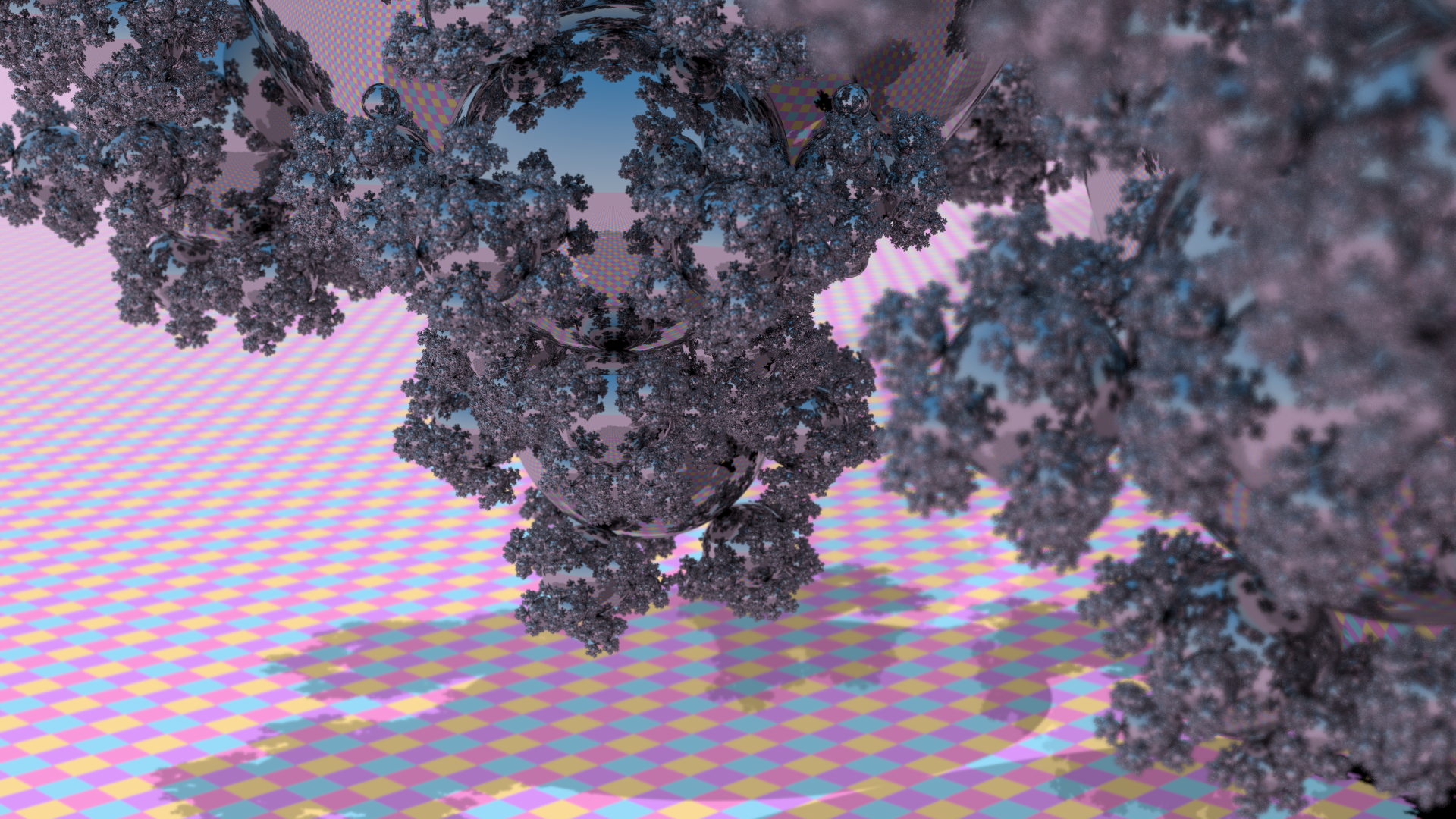
I decided to see how far I could push the system before it broke. 30-odd years ago I made a ray tracing benchmark suite, the Standard Procedural Databases (called that mostly so I could use the acronym SPD). I created one model I dubbed “sphereflake.” It is sort of a 3D Koch snowflake, a fractal curve that defines a shape with a finite area but infinite perimeter. Similarly, at each level of the sphereflake, the radius of the spheres is a third of that of the parent sphere. With nine children for each parent, each new level of recursion adds in the same amount of surface area as the level before. This makes for a model that, taken to its limit, has a finite volume (1.5 times that of the initial sphere) and an infinite surface area. The material model is simpler than that used in Chris’s and Pete’s tutorial scene: just a diffuse plane (which we all fake with a giant sphere) and reflective spheres.
Figure 2 shows sphereflake with a hemispherical light source:
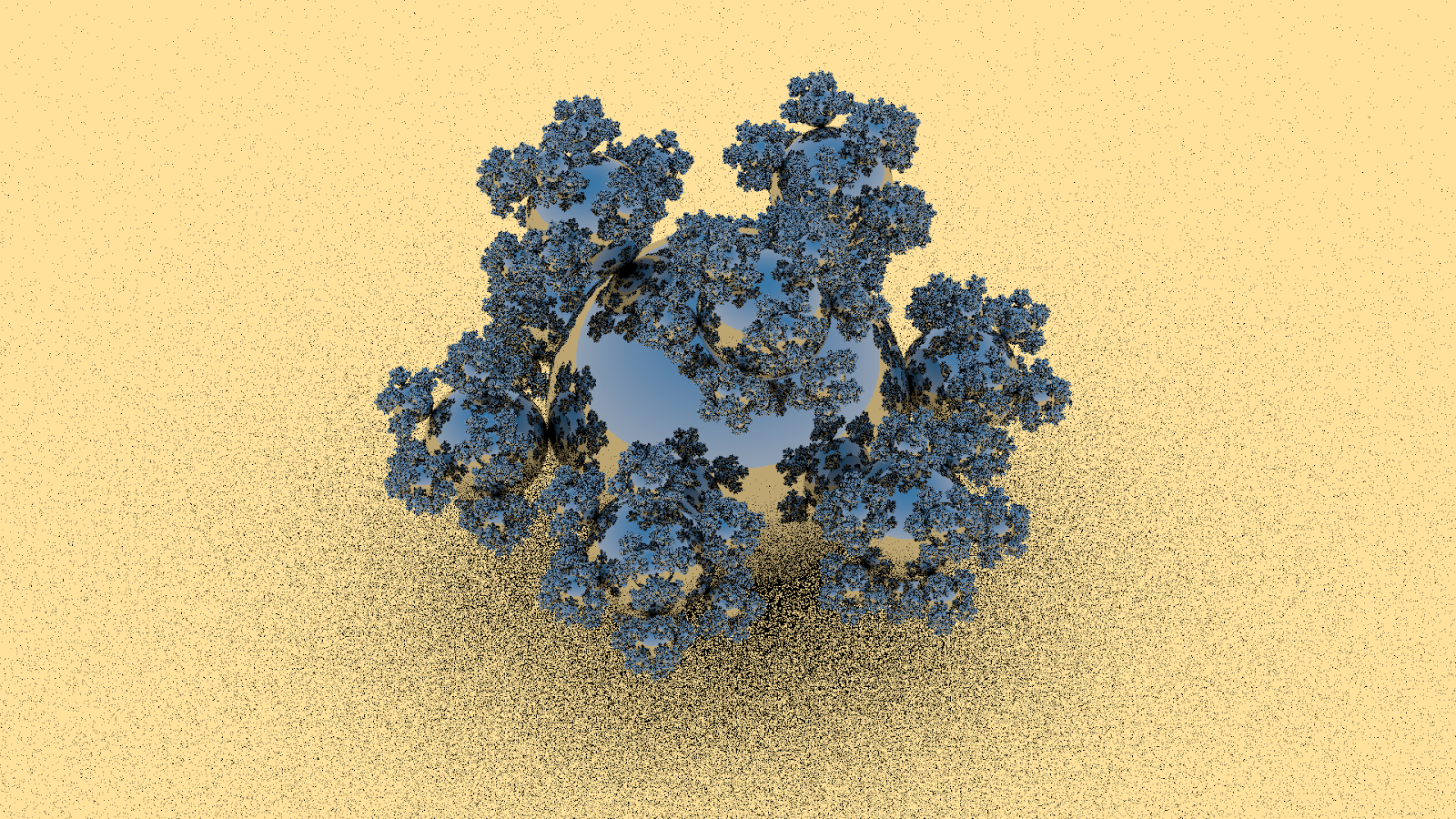
The huge area light causes noise, since a single shadow ray is shot at each ground location in a random direction. Some rays hit the sphereflake, causing a shadow.
After a minute of convergence things look fine, as we see in figure 3:
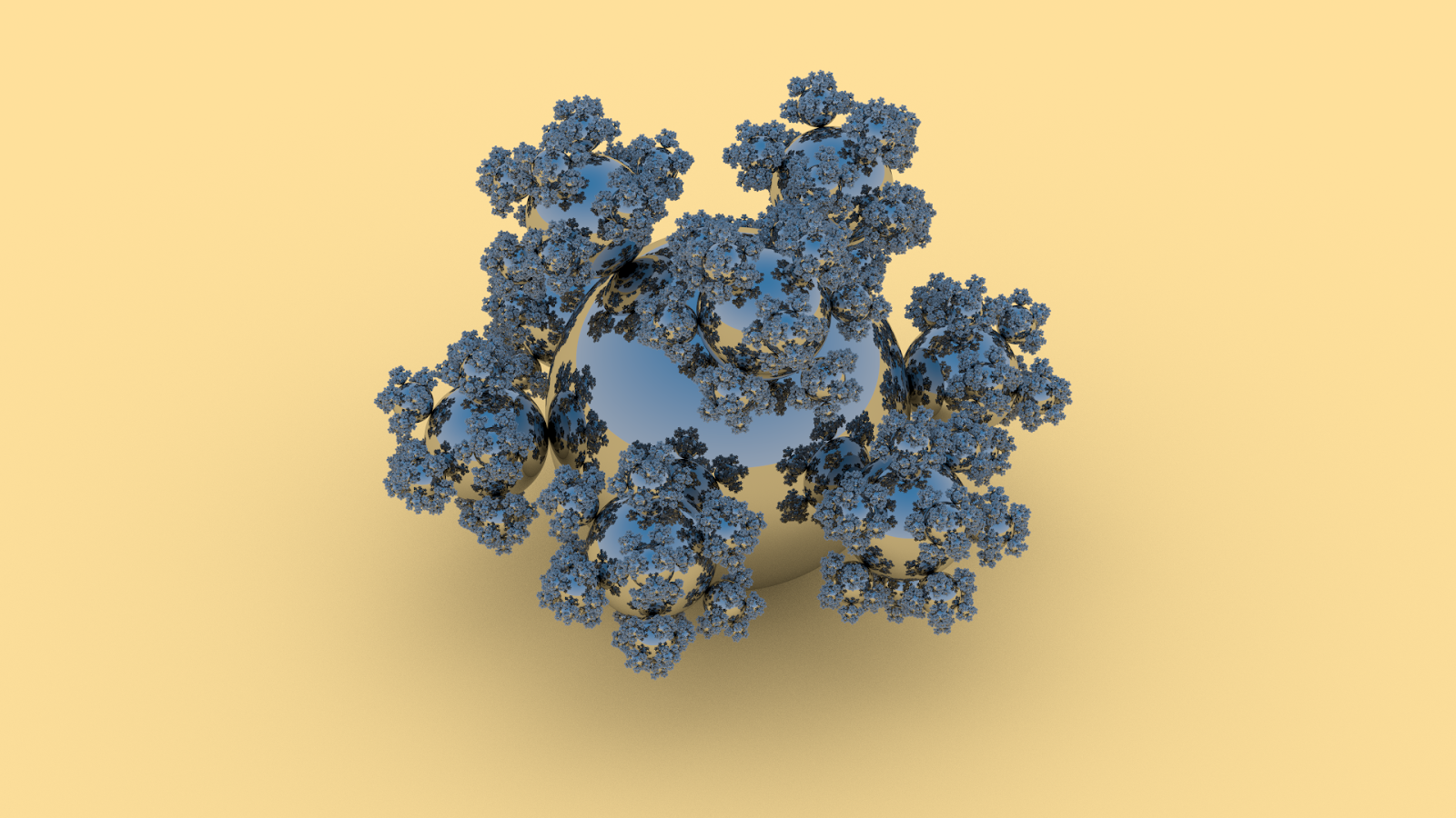
The reflections look good, and it’s enough to go 5 levels deep (spheres reflecting spheres reflecting…). Also, and this was the first “Wow!” moment for me, I could push the procedural model creator up to 8 levels, meaning that we’re rendering 48 million (48,427,562 exactly, since you asked) spheres. Level 9, 436 million spheres, is outside the range for a single Titan V or RTX 2080 Ti.
However, I created a separate object for each sphere. Steve Parker pointed out that I could use instancing, which should conservatively give me 20.8 trillion spheres. Maybe I’ll try this next week, though realistically the scene already has a ratio of 24 spheres per pixel right now and the smallest spheres are mostly twinkly noise when I move through the scene.
But, I can move through the scene! From this view I was getting 90 FPS at a resolution of around 1920 x 1080! Back in 1986 I was rendering 7,382 spheres which took well over an hour to render a 512 x 512 test scene. The sheer number of objects I can render in real-time is honestly mind-blowing for me. Before doing this experiment I thought, “Well, Chris’s 433 sphere demo was snappy, but 7.3k shiny spheres will probably kill performance – here’s hoping it’s still interactive.”
NVIDIA’s CEO likes to quote 10 GigaRays/sec for Turing. Me, I like to quote 48 million spheres. And don’t even think about how many triangles that would be if tessellated and rasterized, not to mention forget about local reflections. Note that all rendering here is pure ray tracing throughout. Most of Chris’s tutorials use rasterization for the initial eye rays, as rasterizing these can normally beat ray tracing for performance. Not so for scenes with custom primitives such as spheres.
Less, Less!
A hemispherical light dome gives a lovely soft shadow after a while, but is much more circa 1986 – path tracing and The Rendering Equation – than 1980 – classic Whitted ray tracing with sharp reflections, refractions, and shadows. I wanted to implement three directional lights for the scene, which is how it was originally designed. This turned out to be a snap. Let’s look at the older shader code first:
float3 randDir = getCosHemisphereSample(randSeed, N);
float isVisible = shootShadowRay(hit + N * 0.001f, randDir);
The new code:
float3 light1 = float3(-0.507093, 0.845154, -0.169031);
float3 light2 = float3( 0.174078, 0.696311, 0.696311);
float3 light3 = float3( 0.742781, 0.371391, -0.557086);
float isVisible =
   shootShadowRay(hit + N * eps, light1) * saturate(dot(N, light1))
   + shootShadowRay(hit + N * eps, light2) * saturate(dot(N, light2))
   + shootShadowRay(hit + N * eps, light3) * saturate(dot(N, light3));
(Pro tip #2: if you change an .hlsli file in these demos, hit “F5” and move the view to reload. This feature makes shader development ridiculously fast.)
Shoot three shadow rays, multiply by the effect of each light compared to the surface normal, and you have shadows, as figure 4 shows:
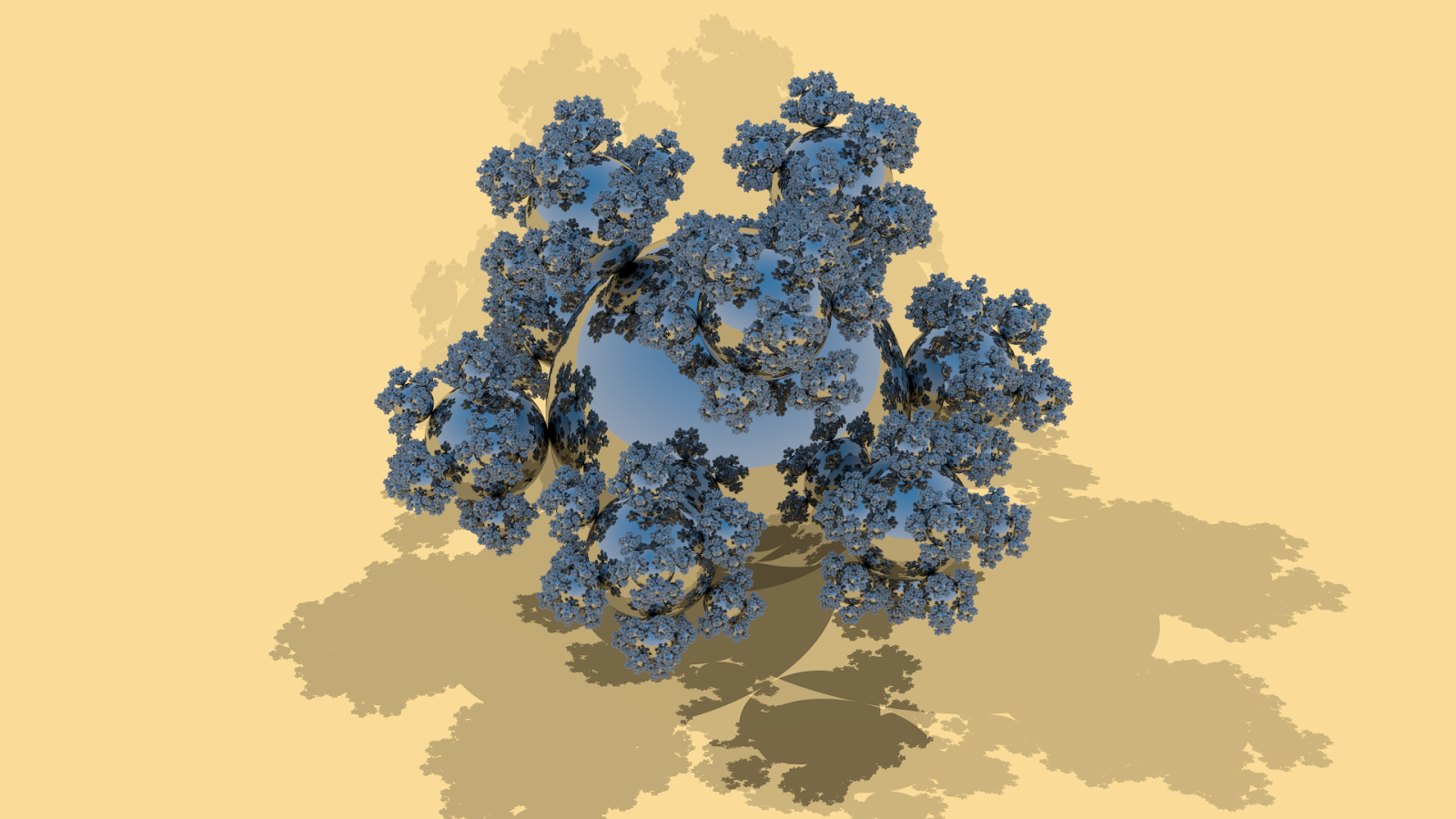
Those shadows are sharp while moving around, not noisy. For this view I get about 60 FPS – lower than before, since I’m shooting three shadow rays instead of just the random one for the hemispherical light. If I zoom in, so that everything is reflecting and spawning a lot of reflection rays (and fewer shadow rays, as I don’t compute shadows for entirely reflective surfaces), it drops to no lower than 30 FPS.
I mentioned these stats to Tomas Akenine-Möller, who had just received an RTX 2080 Ti. I wasn’t sure this new card would help much. RT Cores accelerate bounding volumes, sure, but they also include a dedicated triangle intersector that won’t get used. He runs the demo at 173 FPS for the view above, and 80-90 FPS for a zoomed-in view, such as the one in figure 5:

Now I’m sure.
Forward to 1984
While a bad year for Winston Smith, 1984 was a great year for graphics. For example, that year saw the introduction of Radiosity. Pixar had a bunch of wonderful papers, including one by Rob Cook and all on what they called “distributed ray tracing” (and that everyone else eventually called “stochastic ray tracing”). The idea is simple: shoot more rays to approximate the effect of the material, light, motion, depth of field, etc. For example, to get soft shadows, shoot shadow rays towards random locations on an area light and average the results.
My naive implementation for area light shadows took less than 15 minutes to get working, with a code addition of:
light1 = getCircularAreaSample(randSeed, light1, area);
light2 = getCircularAreaSample(randSeed, light2, area);
light3 = getCircularAreaSample(randSeed, light3, area);
before computing isVisible in the previous code snippet. Most of my work was on getCircularAreaSample, which I derived from the hemispherical light’s getCosHemisphereSample subroutine, using a radius for the directional light’s area.
Adding a slider to the demo, I could now vary the lights’ radii as I wished, and so had soft shadows, with variations shown in figures 6 and 7:


The images seen here are the results after a few seconds of convergence. The softer the shadow, the more rays that need to be fired, since the initial result is noisy (that said, researchers are looking for more efficient techniques for shadows). I did not have access in these demos to denoisers. Denoising is key for interactive applications using any effects that need multiple rays and so create noise.
What impressed me about adding soft shadows is how trivial it was to do. There have been dozens of papers about creating soft shadows with a rasterizer, usually involving clever sampling and filtering approximations, and few if any of them being physically accurate and bullet-proof. Adding one of these systems to a traditional renderer can be person-months of labor, along with any learning curve for artists understanding how to work with its limitations. Here, I just changed a few lines of code and done.
I borrowed one more feature from the “Weekend” demo: depth of field. Vary the starting location on the virtual lens to go through a focal point and you have the effect. Turn this on for Sphereflake and add a procedural texture. You get the result seen in figure 8:
The shadows here are actually hard-edged again, but the depth of field effect blurs the distant one in particular, along with the ground texture.
Now What?
Adding some effects to a ray tracer is dead simple, and addictive. For example, I’ve held myself back from adding glossy reflections; perhaps you want to add these yourself? As for me, I began collecting ray tracing related links again, after a eight-year hiatus from publishing the Ray Tracing News.
If you recently got a Turing-based card, you can grab the code here. You can try toying with the shaders or making entirely new demos. These tutorial programs are built atop Falcor and are focused on letting you modify shaders. After decades of lock-step Z-buffer rendering, being able to take arbitrary numbers of samples in arbitrary directions is wonderfully liberating. The interactivity and ability to handle a huge amount of geometry is still sinking in.