One of the most common challenges with big data is the ability to merge data from several sources with minimal cost and latency. It’s an even bigger challenge merging from various streaming sources in near-real time—along with batch logs data—in a continuous fashion.
At NVIDIA, GeForce NOW is a cloud game-streaming service where users can play games from anywhere on any PC, Mac, or NVIDIA Shield devices. It is a complex service with several microservices working together to provide the best gaming experience.
The use case is to build a data platform that can ingest data from all these microservices and merge them based on a common identifier. This enables the engineering, operations, and business teams to build real-time analytics, actionable alerts, visualizations, and reports; perform correlation analysis; and easily create datasets for machine learning models.
Because the data is already merged, individual users need not worry about knowing the raw data schema or optimizing queries. It provides a seamless, self-serve platform addressing multiple use cases. If you have a question in mind, it only takes a few clicks to analyze the data and get answers.
Here is the story of how NVIDIA used Apache Spark stream-stream joins and watermarking features and reduced the end-to-end latency from three hours to 15 minutes. We did not blow up the costs and also successfully addressed scalability and reliability requirements.
Objectives
In a broader sense, our objectives are defined for two types of users:
- Microservice developers who need a self-serve platform for adding or updating metrics as their microservices evolve.
- Data analysts and data scientists who consume the metrics for building models and making key conclusions.
For both user types, the platform should be easy to operate and maintain, scalable, reliable, low-cost, and low-latency.
Challenges
A session in GeForce NOW starts when a user clicks play on the client and ends when the user exits the game. We want to capture all the events and metrics related to the session and create a session document that provides a holistic view of what happened.
This session document includes data from all the microservices. Microservices use a push model to send telemetry and logs. Telemetry is sent in real time throughout the session and logs are sent at the end of the session, which means that data arrives at different time periods.
The challenge here is to merge data as it becomes available and the session document is updated in near-real time. Another challenge is that both telemetry and logs data can be either structured or unstructured, and change over time. The volume of data is very large, and thousands of metrics must be computed to build the session document. Also, most big data systems are not meant for handling upserts, so this also has to be factored into the design.
Architecture
Our big data platform primarily consists of the following services:
- Apache Kafka as the message queue
- Apache Spark for compute
- Amazon S3 for storage
- Delta Lake on Databricks as the data warehouse
- Elastic for search, analytics, and alerting
Figure 1 shows the overall flow of data and different components of the platform.
Several other tools are built around these services for monitoring, cost-tracking, authentication, continuous integration and delivery, GDPR compliance, performance optimization, and retention management.
On the Elastic side, we use Kibana for visualizations and dashboards and Watcher for alerting. On the Spark data warehouse side, we use Tableau for visualizations and dashboards, and DBeaver for running ad-hoc queries.
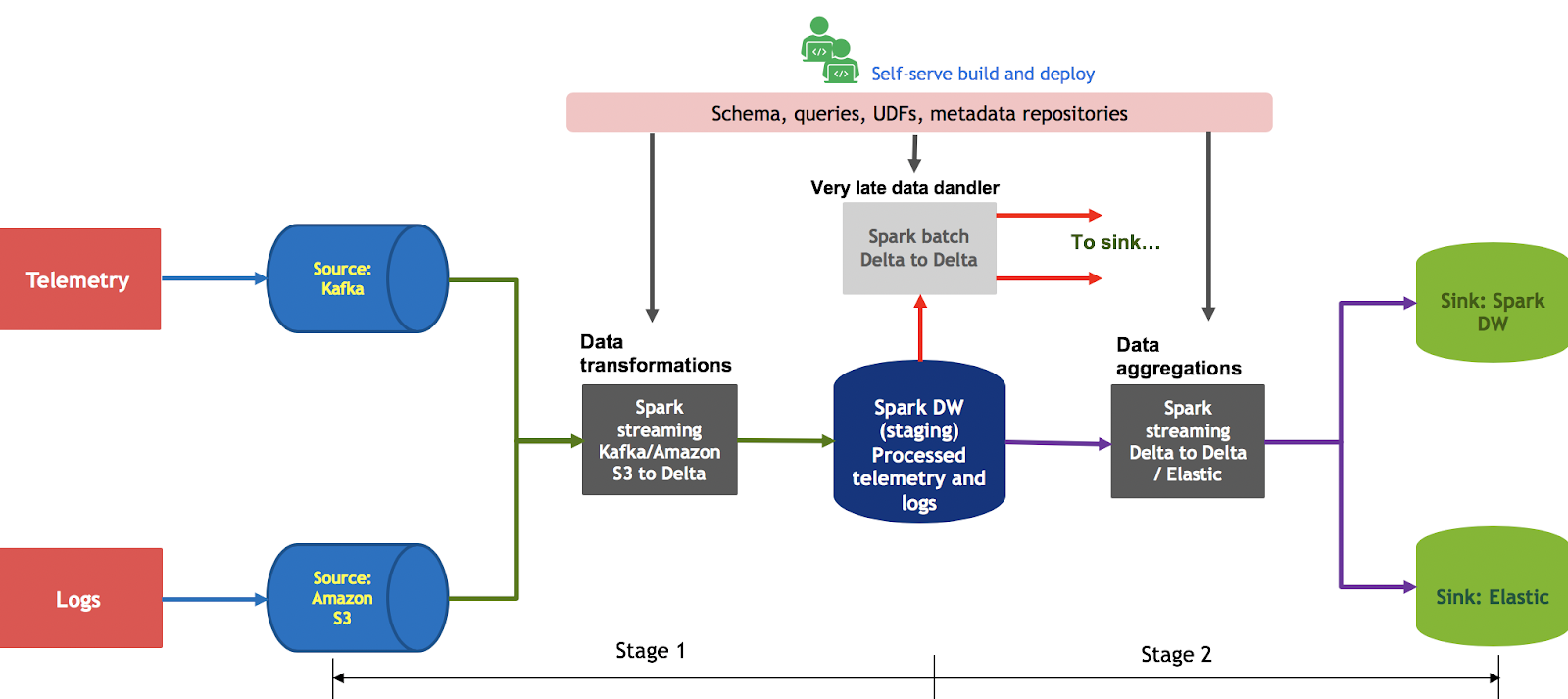
Before we decided on this architecture, we were using Spark batch jobs for all data processing in this pipeline. Several drawbacks included high latencies, cost, limited self-serve capabilities, scalability, and high stress on Elastic resulting in reliability issues. This motivated us to design a streaming pipeline to address all these issues. All the telemetry data is pushed to Kafka from an API gateway and all the logs are copied to Amazon S3 from multiple Availability Zones distributed globally.
The Spark jobs are divided into two stages. In the first stage, the Spark structured streaming job reads from Kafka or S3 (using the Databricks S3-SQS connector) and writes the data in append mode to staging Delta tables. Each topic in Kafka and each bucket in S3 has its own schema and the data transformations are specific to each microservice. Users can add their business logic using Spark SQL and define their own UDFs.
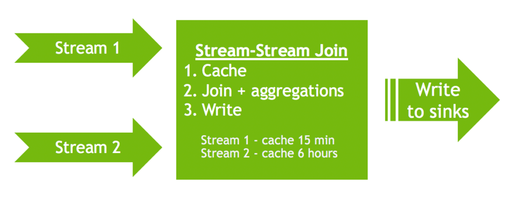
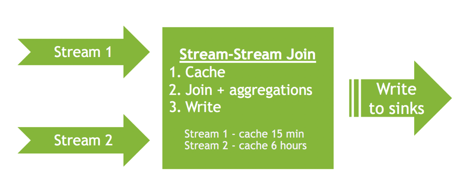
In the second stage, the Spark job reads from Delta Lake tables and performs data aggregations (group by id), drop duplicates, unions, and joins. Here, we primarily use stream-stream joins and watermarking features (see Figure 2) and write to sinks in update/append mode using each batch.
- Update mode allows us to write the data into the sinks when it arrives. For each batch, this ensures that all the sinks are consistent and that users looking at any of the sinks have the same data.
- The watermarking feature stores the data in memory for a certain period of time and performs all the join and group by operations in memory, which is extremely fast. When the watermarking window is crossed, all the old data is flushed from memory automatically.
In this use case, we sync the data in the following ways:
- For writing to the Elastic sink, we write in upsert mode
- For writing to the Delta Lake sink, we use merge into queries
Any data that arrives outside of the watermark window is handled by the late data handler, which reuses the same Spark streaming queries but in batch mode. The two-stage approach isolates source issues and sink issues to specific streaming jobs without affecting the overall pipeline.
We also found that the cost of running a single stage pipeline is more or less the same as running a two-stage pipeline, with the only difference being additional Spark drivers. Also, I should mention that all the experiences shared here are based on PySpark streaming jobs
Optimization
We did several optimizations to find the right balance of cost, reliability, and latency. Thanks to the Databricks engineers for some useful tips.
Using the for each batch writer instead of the native writer to Delta and Elastic
The for each batch writer allows us to do the aggregations and joins one time, writing to multiple sinks
def foreach_batch_function(df, epoch_id):
      df.persist()
      util_write_elastic_batch(df)
      util_write_delta_batch(df)
      df.unpersist()
sink_stream = df.writeStream.outputMode("update") \
      .trigger(processingTime=processing_time) \
      .option("checkpointLocation", checkpoint_location) \
      .foreachBatch(foreach_batch_function).start()
Using unions and group by instead of joins and drop duplicates whenever possible
We found out that using union and group by results in less checkpointing cost than using joins. It is also more efficient because you don’t have to use drop duplicates for any of the streams. This is important if you are checkpointing to Amazon S3.
Spark streaming jobs write to the checkpointing directory with each micro-batch, which results in lots of list bucket calls. This can run into several thousands of dollars just in list bucket cost. For example, if you are joining two streams, you must drop duplicates on both streams, use group by on one of the streams, and then use a join. This results in Spark maintaining four different states for each checkpoint.
Checkpointing to S3
The first two optimization tips reduced our checkpointing costs significantly and we also set minBatchesToRetain to 16 to save on storage costs. We set up a separate S3 bucket to track checkpointing costs. Because of the for each batch writer, we use only one checkpointing directory, although we are writing to multiple sinks.
Writing to sinks in batch mode
One drawback of the first optimization tip is that when one of the sinks is down, the entire Spark streaming job fails. This can be mitigated to a great extent by using retries for writing to Delta Lake. For Elastic, we use the es.update.retry.on.conflict, es.batch.write.retry.count, and es.batch.write.retry.wait options
Shuffle partitions
The Spark default for shuffle partitions is 200 and tweaking this parameter is important for several reasons: It improves the throughput and batch duration, requires fewer workers, and reduces the Amazon S3 list bucket cost.
Trigger processing
By default, Spark starts processing the next micro-batch as soon as the previous one is complete. This requires more workers, and also means more frequent checkpointing or no control over checkpointing.
Setting this to a value greater than batch duration—and an acceptable value to meet the latency goals—significantly reduces the pipeline cost. For example, reducing the shuffle partition from 200 to 32 and setting the trigger processing to be between 60s to 180s reduced our Amazon EC2 cost by 25% and list bucket cost by up to 4X.
Another great use of setting this parameter is not upserting too frequently to Elastic, which otherwise causes performance issues on the Elastic side. This acts as a control knob.
AWS instance types
Using r5.xlarge instances for append mode and i3.xlarge for update mode improves performance and reduces cost.
- Append mode is mostly write-heavy and requires more CPUs and to some extent memory, depending on the data transformations.
- Update mode requires lots of memory for watermarking and in-memory joins and aggregations. An I/O cache-optimized instance is best suited for this mode.
Source- or sink-related optimizations
- Kafka-Spark: Using
maxOffsetsPerTriggerhelps with faster recovery in case of Kafka issues. To improve Kafka and Spark streaming performance, you may also want to play around with the number of partitions per topic. - S3-SQS-Spark: Setting
SET spark.sql.files.ignoreMissingFiles=trueimproves reliability; otherwise, jobs fail if files are deleted in S3. You can play withsqsFetchIntervalandmaxFilesPerTriggerto improve Spark performance. To help reduce storage cost, you can also reducelogRetentionDurationandcheckpointRetentionDurationfor the checkpointing directory. - Delta-Spark and Spark-Delta: When writing to Delta, a higher coalesce (plus repartition) number helps with faster recovery. This is important when starting the stream after a catastrophic failure with a large backlog to process. For normal operation, setting this to a low value improves the performance of downstream jobs, reduces the cost of optimizing the Delta Lake tables, and requires fewer workers for downstream jobs to maintain higher throughput. Setting this to less than 3 puts too much load on the Spark driver and results in high batch duration. Databricks also released the auto-optimize feature recently, which helps avoid specifying coalesce.
- Delta: Run Optimize and Vaccum as frequently as possible, depending on your cost budget.
- Elastic: We use hot, warm, and cold architectures for the Elastic indices. A hot index is the one where most of the upserts are happening, warm is mostly search-heavy with some upserts specifically during rollover time periods. Cold is search-only with no writes to this index. This allows us to recover faster in case of issues, specifically when there is a sudden influx of data and we have to update the shard count.
Switch and destroy deployment
To minimize downtime, we adopt a switch-and-destroy strategy to deploy updates to streaming jobs. This just means that we start a new cluster, assign jobs to the new cluster, terminate the old cluster, and then start the jobs on the new cluster. This reduces the downtime to less than 3 min. Streams recover faster as well.
We also found that it is safer to terminate the old cluster before starting the new jobs. n some cases, Spark streaming jobs were not stopping gracefully, with some zombie threads lingering around especially for PySpark jobs.
RocksDB state store
Databricks provides an option to use the RocksDB state store instead of the Spark default state store. The RocksDB state store works amazingly well if you have stream-stream joins or group by operations on large datasets with millions of keys and hundreds of columns.
For some use cases, streams were failing after a few days using the Spark default state store. After we switched to RocksDB, streams run for months without any issues. You can enable this by running the following command:
spark.conf.set("spark.sql.streaming.stateStore.providerClass", "com.databricks.sql.streaming.state.RocksDBStateStoreProvider")
Next Steps
We have been running this pipeline for more than six months now without any issues. Our data volume has doubled since its inception and it is rock solid. We are continuing to learn and implement more and more optimization strategies, but at this point I would like to say we have covered 90% of the possible optimization.
Some of the issues we are working around include deploying schema updates, checkpoint incompatibility updates, changing some runtime parameters like coalesce on the fly and other Spark settings without restarting the clusters, and minimizing delays due to these deployments.
This pipeline has been successfully handling 5X loads and scales without any issues. We are going beyond 5X soon and it will be interesting to see how it scales and performs. We also implemented built-in monitoring to track lag, latency, and throughput, and self-serve deployment for all the streaming jobs. The latter deserves a separate post by itself.
I’d like to thank Amit Singh Hora and all the team members who contributed to the development of this pipeline.
