Ever looked up in the sky and wondered where it all came from? Cosmologists are in the same boat, trying to understand how the Universe arrived at the structure we observe today. They use supercomputers to follow the fate of very small initial fluctuations in an otherwise uniform density. As time passes, gravity causes the small fluctuations to grow, eventually forming the complex structures that characterize the current Universe. The numerical simulations use tracer particles representing lumps of matter to carry out the calculations. The distribution of matter at early times is known only in a statistical sense so we can’t predict exactly where galaxies will show up in the sky. But quite accurate predictions can be made for how the galaxies are distributed in space, even with relatively simplified simulations.

As observations become increasingly detailed, the simulations need to become more detailed as well, requiring huge amounts of simulation particles. Today, top-notch simulation codes like the Hardware/Hybrid Accelerated Cosmology Code (HACC ) [1] can follow more than half a trillion particles in a volume of more than 1 Gpc3 (1 cubic Gigaparsec. That’s a cube with sides 3.26 billion light years long) on the largest scale GPU-accelerated supercomputers like Titan at the Oak Ridge National Laboratory. The “Q Continuum” simulation [2] that Figure 1 shows is an example.
While simulating the Universe at this resolution is by itself a challenge, it is only half the job. The analysis of the simulation results is equally challenging. It turns out that GPUs can help with accelerating both the simulation and the analysis. In this post we’ll demonstrate how we use Thrust and CUDA to accelerate cosmological simulation and analysis and visualization tasks, and how we’re generalizing this work into libraries and toolkits for scientific visualization.
An object of great interest to cosmologists is the so-called “halo”. A halo is a high-density region hosting galaxies and clusters of galaxies, depending on the halo mass. The task of finding billions of halos and determining their centers is computationally demanding.
Finding Halos
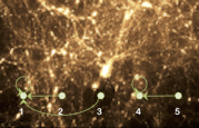
One commonly used method of finding a halo is “friends-of-friends”, in which any two particles within a specified “linking length” of each other are joined into the same halo. Friends-of-friends halos can be identified efficiently using a KD-tree based algorithm.
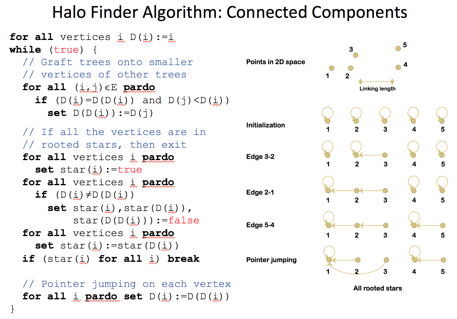
An alternative approach is to interpret finding friends-of-friends halos as finding connected components of a graph where the vertices are the particles and an edge exists between two particles if and only if the distance between them is less than the linking length. Figure 2 shows pseudocode for a standard sparse parallel connected components algorithm [3].
However, in our case, it is impractical to explicitly compute and store all the edges of this graph as in the example above. We therefore use a spatial partitioning to map each particle to a cell, and re-compute the edges on the fly by searching neighbor cells for particles within the linking length of a given particle.
This data parallel algorithm maps nicely to the primitives offered in the Thrust library. The following example code uses Thrust to implement the core of the sparse parallel connected components algorithm, with spatial partitioning. The calls to for_each take user-defined functors (such as graft_p) that implement the specifics of the parallel operations.
// Preconditions: Particles have been sorted by bin id, which is contained in B;
// start and end of search ranges for each particle are in N1 and N2 (each of length 9*n);
// coordinates for each particle's location are in X, Y, and Z; D tracks the parent id for
// each particle, initialized to itself; F contains a flag for each neighbor indicating
// whether it needs to be searched

// Iterate until all vertices are in rooted starsOPTnumber = {number},
while (true) {
  // Graft trees onto smaller vertices of other trees
  thrust::for_each(thrust::make_counting_iterator(0),
                   thrust::make_counting_iterator(0)+n,
                   graft_p(n, num_bins_x, num_bins_y, num_bins_z, bb,
                           thrust::raw_pointer_cast(&*D.begin()),
                           thrust::raw_pointer_cast(&*X.begin()),
                           thrust::raw_pointer_cast(&*Y.begin()),
                           thrust::raw_pointer_cast(&*Z.begin()),
                           thrust::raw_pointer_cast(&*B.begin()),
                           thrust::raw_pointer_cast(&*N1.begin()),
                           thrust::raw_pointer_cast(&*N2.begin()),
                           thrust::raw_pointer_cast(&*F.begin())));

  // Compute which vertices are part of a rooted star
  thrust::fill(S.begin(), S.end(), true);
  thrust::for_each(thrust::make_counting_iterator(0),
                   thrust::make_counting_iterator(0)+2*n,
                   is_star1(thrust::raw_pointer_cast(&*D.begin()),
                   thrust::raw_pointer_cast(&*S.begin())));
  thrust::for_each(thrust::make_counting_iterator(0),
                   thrust::make_counting_iterator(0)+2*n,
                   is_star2(thrust::raw_pointer_cast(&*D.begin()),
                            thrust::raw_pointer_cast(&*S.begin())));

  // If all vertices are in rooted stars, algorithm is complete
  bool allStars = thrust::reduce(S.begin(), S.end(), true, thrust::logical_and());

  if (allStars) { break; }
  else {          // Otherwise, do pointer jumping
    thrust::for_each(thrust::make_counting_iterator(0),
                     thrust::make_counting_iterator(0)+2*n,
                     pointer_jump(thrust::raw_pointer_cast(&*D.begin())));
  }
}
Using the magic of Thrust, this is now a massively parallel, GPU-accelerated implementation of a halo finder.
Finding Halo Centers
In addition to finding the particles belonging to halos, the centers of the halos needs to be found. The most bound particle (MBP) is often defined as the halo center, and is computed by finding the particle with the minimum potential, where the potential for a particle depends on its distance from all other particles in the halo.
We compute the most bound particle for a single halo using thrust::for_each() with a functor that computes the potential for a particle by computing its distance to all other particles, followed by a forward and a reverse thrust::inclusive_scan() with the minimum function object to propagate the minimum potential value to all particles in the halo. We then use thrust::transform() to identify the index of the particle whose potential is equal to the minimum value, followed by another forward and reverse inclusive_scan() to propagate that index to all other particles in the halos. If there is sufficient memory available, MBPs can be found for multiple halos simultaneously by using the segmented version of the Thrust scan (inclusive_scan_by_key()), with the halo IDs as the keys.
PISTON Visualization and Analysis Library
The original center-finding code in HACC relied solely on MPI for parallelism, with serial computation within each MPI rank. However, in our specific case, memory constraints due to the overload zones and limitations of OpenCL prevented us from running more than one MPI rank per node. This provided even greater motivation to utilize the computing power of Titan’s GPUs for this analysis task.
Instead of writing a stand-alone halo finding application on top of Thrust, we chose a slightly more general approach. While some people might view halo finding to be part of the main simulation, we decided that this was part of the visualization and analysis system. We therefore wanted to extend our visualization system with a mechanism to handle data structures resident on the GPU and treat halo finding in the same way as (for example) smoothing a data volume, or any other filter.
In fact, over the last few years, we have been writing a wide variety of visualization and analysis operators using the Thrust library. We have found Thrust to be a very useful tool for this library, which we call “PISTON”, since it allows us to quickly write algorithms that can run both on multi-core CPUs and on NVIDIA GPUs, without having to write any low-level CUDA code. The data-parallel algorithms provided by Thrust (such as scan, reduce, transform, and sort) correspond nicely to the “scan vector” model proposed by Guy Blelloch (“Vector models for data-parallel computing”, PhD thesis, MIT, 1990), and can be used as building blocks for a wide array of algorithms.
Kitware has also developed a ParaView plug-in to allow PISTON to be called from ParaView and Catalyst, so that it can be used not only for post-processing but also for in-situ visualization and analysis. Our PISTON halo finder has also been integrated into the CosmoTools library, which is used for in-situ visualization and analysis within HACC.
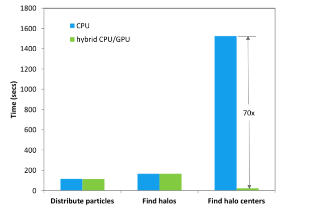
Using Piston, we were able to significantly accelerate the analysis of the simulations.
Figure 3 shows the results on Titan for a 10243 particle run on 32 nodes, with the same mass resolution as the 81923 particle run mentioned in the introduction. The speedup for MBP center finding was about 70x when compared to the CPU version of the algorithm using one MPI rank per node on Titan. Center finding is much more time consuming than halo finding, and our speed-ups for finding halos were not as large as for finding centers (since the halo finding algorithm is not work-optimal), so, for the Q Continuum simulation run, we used a hybrid approach using Thrust code on the GPU for center finding but the original CPU code for the halo finding.
From Piston to VTK-m
The development of Piston was made possible by the US Department of Energy, as part of the SDAV SciDAC center, as well as the DOE Advanced Simulation Computing Program. The goal of the SDAV SciDAC center was to investigate novel approaches to data analysis and visualization and methods of exploiting massive parallelism.
Within this center, our “PISTON” library of visualization and analysis algorithms, implemented using Thrust, has merged with two related efforts (Dax at Sandia National Laboratory and Kitware, and EAVL at Oak Ridge National Laboratory) to form “VTK-m”. VTK-m, currently in development, will be a new version of the popular Visualization Toolkit (VTK) library that takes advantage of the parallelism available on multi-core and many-core accelerators, such as GPUs, for computation (not just rendering). This project involves the development of a new, more flexible data model, an execution model that efficiently supports running on a variety of architectures, and a library of common visualization and analysis operators written on top of this data and execution model.
References:
- Habib et. al., ‘HACC:Simulating Sky Surveys on State-of-the-Art Supercomputing Architectures’, New Astronomy (in print)
- Heitmann et. al., ‘ The Q Continuuum Simulation:Harnessing the Power of GPU Accelerated Supercomputers’, ApJSupp (submitted)
- J. JaJa. An Introduction to Parallel Algorithms. Chapter 5, pages 204–222. Addison-Wesley, 1992.