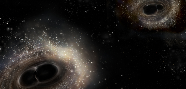
GPU-Accelerated Black Hole Simulations

In February 2016, scientists from the Laser Interferometry Gravitational-Wave Observatory (LIGO) announced the first ever observation of gravitational waves—ripples in the fabric of spacetime. This detection directly confirms for the first time the existence of gravitational radiation, a cornerstone prediction of Albert Einstein’s general theory of relativity. Furthermore, it suggests that black holes may occur in nature considerably more commonly than anticipated, and pioneers an entirely new form of astronomy based on direct observations of gravity rather than of light.

Artist’s illustration of the merging binary black hole systems GW150191 (left) and GW151226 (right). Image Courtesy Caltech/MIT/LIGO Laboratory. Ccredit: LIGO/A. Simonnet. — Artist’s illustration of two merging binary black hole systems GW150191 (left) and GW151226 (right). While they are portrayed together here, these two merging systems were detected at different times and in different parts of the sky. Image courtesy Caltech/MIT/LIGO Laboratory. Ccredit: LIGO/A. Simonnet.

The LIGO Laboratory operates two detector sites, one near Hanford in eastern Washington, and another near Livingston, Louisiana. This photo shows the Livingston detector site. Image Courtesy Caltech/MIT/LIGO Laboratory.

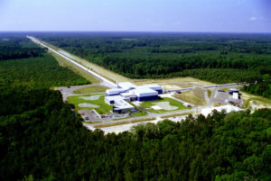
The gravitational wave experiment LIGO has now reported the first few detections (of many to come) of the gravitational radiation from binary black holes (BBH: a pair of closely orbiting black hole). These detections are made by firing lasers at mirrors at the ends of two widely separated perpendicular tunnels, called “arms”: upon return from the mirrors, the interference pattern generated by the lasers measures the relative length of the arms. Since gravitational waves contract and expand the arms at different rates, the waves can be measured by studying the fluctuations in the interference pattern.

Unfortunately many other things can expand and contract the arms besides gravitational radiation, such as thermal fluctuations in the mirrors, traffic, and in one (perhaps apocryphal) incident, rifle fire directed at the experiment by bored rural Louisianans. The original detection GW150194 was an exception: the typical gravitational wave signal is expected to be far too much weaker than this noise to be visible within the LIGO data stream to the naked eye.

LIGO scientists instead extract the signal using a technique called matched filtering. First, a template bank of predicted gravitational waveforms from binaries of different system parameters—different masses and spins—is generated. The correlation between each template in the bank and each segment of the actual experimental data stream is then computed. Roughly, if a particular template’s correlation exceeds a threshold value, that template can be said to lie within the data, and a binary system has been detected.

For this to work, we need very accurate predictions of the gravitational radiation from binaries of differing system parameters to serve as templates. Newtonian gravity is too inaccurate for this purpose (in particular, it predicts no gravitational radiation). The system needs instead to be modelled using the full machinery of general relativity (GR). But the problem is far too complicated for simple pen-and paper techniques. We thus must integrate the full nonlinear Einstein equations numerically.

Here are the Einstein equations in their four-dimensional presentation:

$R_{\mu\nu} - \frac{1}{2}Rg_{\mu\nu} = \frac{8\pi G}{c^4}T_{\mu\nu}$

The objects on the left-hand side encode the curvature of spacetime. In “flat” spacetime (with zero curvature) two small rocks released at a small initial separation will follow a straight line through spacetime: time will progress forward, but their position in space will not change. In “curved” spacetime (with non-zero curvature) the rocks will instead follow a curved path, so their position in space will change with time. That’s a fancy way of saying that “the rocks will fall”. Thus curvature encodes the effects of gravity.

The right-hand side encodes the matter content of spacetime. One way for the curvature to be non-zero is thus for the right-hand side to also be non-zero: for spacetime to contain matter. In that case the spacetime will curve in such a way as to bend the little pebbles towards the matter. Thus, matter gravitates.

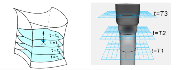
The Einstein equations in this form describe the entire spacetime geometry across both space and time. This is elegant, but not particularly useful for numerical purposes. We need to instead cast the equations into a 3+1 formulation which allows them to be solved as an initial value problem. To do this, we divide 4-dimensional spacetime into a stack of 3-dimensional spatial slices, each corresponding to a particular “moment” in time, as Figure 1 shows. There are an infinite number of ways to cut spacetime up, some of which will behave better numerically than others, but we need to pick one to do the simulation.

Figure 1: Schematics of the 3 + 1 formulation — Figure 1: Schematics of the 3+1 formulation. Left: spacetime (represented as the three-dimensional figure) is divided into spatial slices (the two-dimensional blue sheets). Each slice is labelled by a particular moment in time. Alternative slicings are possible: this reflects the freedom in general relativity to choose which events in spacetime are “simultaneous” with one another. The dot at t=t3 shows a particular event, and the double cone encloses the other events causally connected to that one. The dotted line shows the trajectory of a particular observer through spacetime. Right: a black hole’s event horizon (the grey surface) appears as a lower-dimensional object on each slice. Image credit: Prayush Kumar.

Post-slicing, the Einstein equations break into a system of four (groups of) PDEs. There are many equivalent such systems; here is one of them (the so called “ADM equations”: physically, but not numerically, equivalent to the ones we actually solve):

$R + K^2 - K_{ij}K^{ij} = 16\pi e$
$D_jK^j_i - D_iK = 8\pi j_i$
$\partial_t K_{ij} = -D_i D_j \alpha + \alpha(R_{ij} - 2K_{ik}(R_{ij} - \frac{1}{2}\gamma_{ij}(S - e))K^{kj} + KK_{ij} - 8\pi\alpha + \mathcal{L}_\beta K_{ij}$
$\partial_t \gamma_{ij} = -2\alpha K_{ij} + \mathcal{L}_\beta \gamma_{ij}$

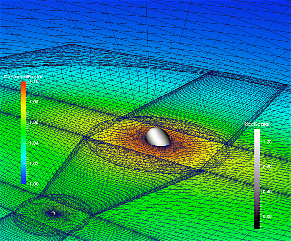
It’s beyond the scope of this post to define all these symbols, but it is worth pointing out that the equations come in two groups. The first two do not depend directly on time and are mathematically elliptic PDEs. They are known as the constraint equations because they constrain the gravitational field of each time slice. If they are violated at any moment, the field at that moment is not allowed by general relativity. Therefore, by solving the constraints, we can obtain initial conditions for our simulation. Figure 2 shows an example.

Figure 2: Initial data for a BBH simulation. — Figure 2: Initial data for a BBH simulation at mass ratio 10 (one black hole 10 times more massive than the other). The colours on the simulation volume show a measure of the local curvature of space, while those on the holes themselves show a measure of the horizon’s curvature. A slice of the simulation grid is overlaid. Note the difference in fineness of the grid near the smaller and larger holes. This is one of the reasons why simulations involving large mass ratios are difficult. Image credit: Harald Pfeiffer.

The second two ADM equations involve time directly and are mathematically hyperbolic. We call them the evolution equations because they, given a gravitational field which satisfies the constraint equations at some time, determine how that field evolves for all times. Thus, by integrating these equations we can find the future state of the field and model the black hole merger.

This sets the essential program. First, we choose masses, spins, separations, and orbital speeds for the black hole binary. Next we solve the constraint equations to find a valid initial BBH configuration with those parameters. Finally, we integrate the evolution equations forward to find how the BBH appears in the future. We can then extract the gravitational waveform from the simulation and compare it to experimental data.

The following three videos show visualizations of simulations meant to model GW150914 (first, second), the first inspiral detected by LIGO between one 36- and one 29-solar-mass black hole, and the second detection GW151226 (third), which was a merger between one 14.2 and one 7.5 solar mass black hole. The first visualization uses a ray tracing algorithm developed by the SXS collaboration to realistically compute the actual appearance of the black holes in space. The second shows the apparent horizons of the black holes atop a coloured plane visualizing the curvature of spacetime and a vector field showing the trajectories of nearby particles. The third, whichi is of GW151226, shows the frequency and strain of the gravitational radiation from the inspiral as viewed on Earth.

While watching the simulations you may notice the black holes evolve through four essential phases. During inspiral they orbit around one another, emitting gravitational energy which causes their orbit to decay. Eventually the dissipation becomes so fast that the motion is more of a fall than an orbit, and the holes are said to plunge. Quickly following plunge is the merger, when the holes join together into a third, larger black hole which may be highly asymmetric. That hole then radiates its asymmetries away during ringdown, leaving behind an isolated, symmetric black hole remnant.

BBH simulations within a certain parameter range are now fairly routine. There is, unfortunately, an essential problem with using numerical integrations to create a template bank in practice: the simulations are very, very expensive, consuming tens of thousands of FLOPS per grid point per time slice. Even the most computationally friendly regions of parameter space can take days of wallclock time to run, and more difficult simulations take months.

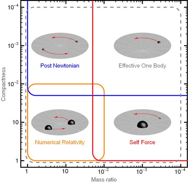
The computational complexity depends importantly on two system parameters. A simulation with a higher mass ratio involves one black hole which is larger than another. Therefore, the simulation must simultaneously resolve two distance scales; this shrinks the simulation time step. Simulations with higher spins, in turn, involve more small-scale fluctuations in the gravitational field; this also shrinks the time step.

Unfortunately, quickly spinning high-mass-ratio systems are among the most interesting to simulate: these systems show the strongest relativistic effects, and furnish easy comparison with analytic theory (see Figure 3). We therefore seek to accelerate the simulations.

Figure 3: Applicability of direct numerical integration (orange box) compared to “pen-and-paper” approximation techniques (red and blue boxes) for two-body mergers. The y scale shows the compactness of the merging objects (denser objects are more compact), while the x shows the mass ratio. To compare with theory we need to perform the very expensive simulations in the overlapping regions. Image credit: Marten van de Meent.

GPU Acceleration

The computations involved in the BBH integration are both highly compute-bound and highly parallelizable. This makes them (technologically) an ideal candidate for GPU acceleration. In practice, however, existing black hole codes are quite difficult to port, simply because the codes are very large and complicated.

We have chosen as target a leading black hole code, the Sppectral EEinstein Code “SpEC”. SpEC employs so-called spectral methods to solve the Einstein equations, which gives favourable algorithmic scaling at the cost of fragility and code complexity. Indeed the code is simply too large to either rewrite from scratch or port line by line.

Thus, we have taken a two-pronged strategy. By profiling the code we first identify “hot spots”: a small number of modules which consume greater than 20% or so of the overall run time. A few of these turn out to be simple enough to write equivalent GPU kernels by hand. Some, however, are not. For these we exploit the fact that our functions can be viewed as linear operations on data. Thus, for each function there exists a matrix $\mathbf{M}$ such that multiplication of the input data by $M$ gives equivalent output.

When the simulation begins we create caches of the matrices $\mathbf{M}$ . When one of the hot spot modules is run for the first time, we trace out the matrix by feeding successive delta functions through the module. Afterwards we can perform the same effect as the module by a simple matrix multiplication, using CUDA-accelerated BLAS operations (cuBLAS). This also improves portability, since CPU BLAS can easily be substituted.

Figure 4: Speedup of GPU-accelerated vs single-CPU version of two “hotspot” modules of SpEC (purple and goldenrod) using the matrix-multiplication approach described above. The black line shows the speedup of the entire code simulating an isolated black hole.In the accelerated version used here, this speedup is limited by kernel launch time of small operations (see below). The comparison to a single CPU is appropriate in our case, since due to scaling constraints and low-level design choices in the code SpEC would replace each single CPU core with an entire GPU. This and all subsequent benchmarks compare a single NVIDIA Tesla M2090 GPU with one core of an Intel Xeon (Sandybridge) E5-2520 2.0GHz CPU.

Tensor Expressions

Having ported the hot spots using hand-written or matrix multiplication kernels we are still left with a large number of smaller operations to be performed on the CPU. This drastically impairs the net speedup since a full CPU-GPU data transfer is thus required at each hot spot. We therefore need some way to keep all the data on the GPU, except at the end of each time step when inter-node communication is required.

Mathematically, the operations we are performing take the form of tensor expressions. Given a vector space, a tensor $T$ is an assignment of a multidimensional array to that space’s basis $\mathbf{f}$ . Should the vector space undergo a change of basis given by a transformation matrix $R$ , a tensor transforms roughly via a multiplication of each component of that array by either $R$ or its inverse. Tensors on more general spaces such as manifolds can then be defined in terms of the tangent spaces to the manifold. For numerical purposes, however, we will view tensors as simply fields of multidimensional arrays, one for each point of the simulation grid.

For example, consider the internal forces—the stress—felt by a small three-dimensional object. Each of three planes through the object ( $xx$ , $xy$ , and $xz$ ) feels a force which itself has three components ( $x$ , $y$ , and $z$ ). Thus to fully describe the stress on the object we need nine numbers: the x-direction force on the $xx$ plane, the y-direction force on the $xy$ plane, etc. It is convenient to bundle these objects together into a single “stress tensor” $\sigma_ij$ .

$i$ and $j$ here are called the indices of the tensor. Each index has a dimension specifying the possible values it may take: in this case the dimension of both indices is 3, since each may take three possible values. The total number of indices in the tensor is called the tensor’s rank. Thus, $\sigma_ij$ is a rank-2 tensor. It may happen to be true that the same number is always obtained when the tensor indices are swapped: $\sigma_ij=\sigma_ji$ . In this case we say the tensor has a symmetry upon the relevant indices.

Tensors of the same rank can be added, multiplied, or divided component-wise. They can also be contracted over an index to produce a new tensor of lower rank. Suppose, for example, that we wish to compute the stress experienced by each plane of an object in some particular direction. We can compute this stress—which will have three components and thus be a rank-1 tensor (a vector) $T_j$ —by contracting $\sigma_ij$ with a vector $n_i$ that points in a particular direction:

$T_j = \sigma_{ij}n_i \equiv \sum_i \sigma_{ij} n_i.$

We express contraction by writing two tensors beside one another with a repeated index: this always implies a sum over that index.

Most operations in a physics code—and certainly in a general relativity code—can be viewed as operations on tensors. Traditionally in an HPC environment we would encode such operations using nested for loops. For example, consider the “index raising” operation, ubiquitous to any general relativity code:

$c_{kj} = a_{ik}*b_{ij}, i,k,j \in 0...N.$ (1)

The above operation might be implemented in C using code like the following.

for (int j=0; j<N; ++j) {
  for (int k=0; k<N; ++k) {     \\*
    double sum=0;
    for (int i = 0; i < N; ++i) {
      sum += a[i][k]*b[i][j];
    }
  }
}

These loops are tedious and hard to maintain. For example, suppose that we wished to express the same operation upon a $b_ij$ with a symmetry (so $b_ij = b_ji$ ): this would amount to replacing the line of code marked \\* above with the following line.

for (int k=0; k<j; ++k) {

This is a very subtle change which can be easily missed while debugging. Such errors become difficult to spot as the complexity and number of expressions increases, and worse, they often compile normally. Creating and maintaining a CUDA port of such code greatly magnifies the difficulty.

On the other hand, given an arbitrary tensor expression, the appropriate code block in either C or CUDA is actually sufficiently predictable that its generation can feasibly be automated. In our original approach to this problem we used C++ expression templates to automatically port the array operation within the for loop to the GPU. Each operation instantiates a templated class BinaryOp<LHS, OP, RHS>, which in the above case would take the following form.

BinaryOp<Array, Assign, BinaryOp<Array, Multiplication, Array>>

Such expressions can be automatically ported to the GPU by compiling the code into a library, linking to an executable that loops over each unique BinaryOp in the library and generates a CUDA kernel from each, then linking those kernels back to a second compilation. Because all computations can via this approach be performed on the GPU, it is no longer necessary to perform repeated CPU-GPU synchronizations. This creates, however, a different problem, illustrated in Figure 5: the sheer number of CUDA calls becomes so large that call latency impairs the overall runtime dramatically.

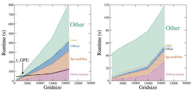
Figure 5: Wall clock time in seconds of SpEC simulating an isolated black hole on a single CPU without (left) and with (right) GPU. The total GPU-accelerated runtime is overlaid upon the CPU plot (black line marked t_GPU). The stacked coloured regions show the contribution to the overall run time of selected “hot spot” modules. The green region shows the contribution from the rest of the code.

Notice in particular how the relative size of the shaded green region has increased in GPU-SpEC (right). Also notice that the scaling of this region is roughly constant. This region is dominated by kernel launch overhead of the many small ported operations described above: each iteration of the loop suffers about 20 microseconds of GPU latency, which ends up dominating the overall run time.

We thus need to bundle our operations together into larger units. To this end we have developed a C++ package, “TenFor”, enabling expressions syntactically very similar to (1) to be written directly into C++ source code. In this way we can avoid the for loops entirely. Using TenFor, (1) is expressed directly in source code as

c(k_,j_) = Sum(a(i_,k_)*b(i_,j_));

While its symmetric equivalent would be

c(Sym<0,1>, k_, j_) = Sum(a(Sym<0,1>, i_, k_)*b(i_,j_));

These expressions are presented to the compiler as a recursive structure of variadic templates, labelling the operations to be performed, the index structures of the tensors, and any relevant symmetries such that mistakes yield errors at worst at link time. In this case, the expression structure would be

TBinaryOp<Tensor, k, j, Assign, TBinaryOp<Null, Sum, <TBinaryOp<Tensor, i, j, Multiply, Tensor<Array<i, j>>>>>

Using a Makefile option, TenFor can be configured to implement expressions in one of three ways. In Nonaccel mode expressions are compiled directly and evaluated using a nested series of expression templates, providing similar functionality to existing tensor packages.

Novel functionality is provided by the other two modes, Accel_CPU and Accel_CUDA. In these modes, user code containing tensor expressions is first compiled into a library that links TenFor. TenFor adds to that library a registry of each unique tensor expression in the source code. The user library is then linked to the TenFor executable CodeWriter, which outputs a C++ (CUDA) function (kernel) from each. These functions are then written to disk as a text file. A second compilation of the user code links the new functions, which perform the operations.

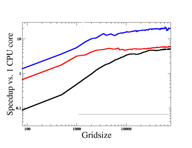
This allows tensor expressions to be written in source code in a compact and maintainable way that directly expresses their mathematical purpose. The expression can be trivially ported from CPU to GPU using CodeWriter, allowing the entire code base to remain on the GPU. In general, the automatically ported code achieves peak efficiency for small, memory-bound tensor operations, with efficiency improving as the operation grows more complex.

Figure 6: Speedup vs 1 CPU core of the operation (1) using Black: automatic porting of individual arrays; Red: TenFor porting, sending pointers to the tensor components to the GPU at each kernel launch time; Blue: TenFor porting, sending pointers to the tensor components once at construction (currently implemented).

Conclusion

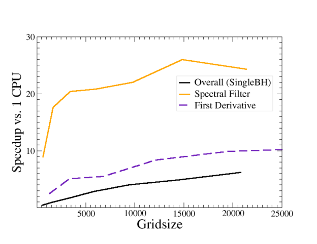
While the full port of the production BBH code is not yet complete, our acceleration of the single black hole test case shows promising results. The rapid porting afforded by the TenFor C++ package has been a big help. We are currently in the process of creating an open-source port of TenFor which does not depend directly upon SpEC. This will be hosted at Bitbucket: https://bitbucket.org/adam_gm_lewis/tenfor.

For more information on gravitational waves and black holes, I recommend you visit the visit the highly informative Simulating Extreme Spacetimes project website, as well as the LIGO homepage.

Thumbnail image courtesy Caltech/MIT/LIGO Laboratory.