

The primary function of NVIDIA TensorRT is the acceleration of deep-learning inference, achieved by processing a network definition and converting it into an optimized engine execution plan. TensorRT Engine Explorer (TREx) is a Python library and a set of Jupyter notebooks for exploring a TensorRT engine plan and its associated inference profiling data.
TREx provides visibility into the generated engine, empowering you with new insights through summarized statistics, charting utilities, and engine graph visualization. TREx is useful for high-level network performance optimization and debugging, such as comparing the performance of two versions of a network. For in-depth performance analysis, NVIDIA Nsight Systems is the recommended performance analysis tool.
In this post, I summarize the TREx workflow and highlight API features for examining data and TensorRT engines.
How TREx works
The main TREx abstraction is trex.EnginePlan, which encapsulates all the information related to an engine. An EnginePlan is constructed from several input JSON files, each of which describes a different aspect of the engine, such as its data-dependency graph and its profiling data. The information in an EnginePlan is accessible through a Pandas DataFrame, which is a familiar, powerful, and convenient data structure.
Before using TREx, you must build and profile your engine. TREx provides a simple utility script, process_engine.py, to do this. The script is provided as a reference and you may collect this information in any way you choose.
This script uses trtexec to build an engine from an ONNX model and profile the engine. It also creates several JSON files that capture various aspects of the engine building and profiling session:
Plan-graph JSON file
A plan-graph JSON file describes the engine data-flow graph in a JSON format.
A TensorRT engine plan is a serialized format of a TensorRT engine. It contains information about the final inference graph and can be deserialized for inference runtime execution.
TensorRT 8.2 introduced the IEngineInspector API, which provides the ability to examine an engine’s layers, their configuration, and their data dependencies. IEngineInspector provides this information using a simple JSON formatting schema. This JSON file is the primary input to a TREx trex.EnginePlan object and is mandatory.
Profiling JSON file
A profiling JSON file provides profiling information for each engine layer.
The trtexec command-line application implements the IProfiler interface and generates a JSON file containing a profiling record for each layer. This file is optional if you only want to investigate the structure of an engine without its associated profiling information.
Timing records JSON file
A JSON file contains timing records for each profiling iteration.
To profile an engine, trtexec executes the engine many times to smooth measurement noise. The timing information of each engine execution may be recorded as a separate record in a timing JSON file and the average measurement is reported as the engine latency. This file is optional and generally useful when assessing the quality of a profiling session.
If you see excessive variance in the engine timing information, you may want to ensure that you are using the GPU exclusively and the compute and memory clocks are locked.
Metadata JSON file
A metadata JSON file describes the engine’s builder configuration and information about the GPU used to build the engine. This information provides a more meaningful context to the engine profiling session and is particularly useful when you are comparing two or more engines.
TREx workflow
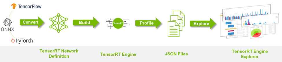
Figure 1 summarizes the TREx workflow:
- Start by converting your deep-learning model to a TensorRT network.
- Build and profile an engine while also producing collateral JSON files.
- Spin up TREx to explore the contents of the files.
TREx features and API
After collecting all profiling data, you can create an EnginePlan instance:
plan = EnginePlan(
    "my-engine.graph.json",
    "my-engine.profile.json",
    "my-engine.profile.metadata.json")
With a trex.EnginePlan instance, you can access most of the information through a Pandas DataFrame object. Each row in the DataFrame represents one layer in the plan file, including its name, tactic, inputs, outputs, and other attributes describing the layer.
# Print layer names
plan = EnginePlan("my-engine.graph.json")
df = plan.df
print(df['Name'])
Abstracting the engine information using a DataFrame is convenient as it is both an API that many Python developers know and love and a powerful API with facilities for slicing, dicing, exporting, graphing, and printing data.
For example, listing the three slowest layers in an engine is straightforward:
# Print the 3 slowest layers
top3 = plan.df.nlargest(3, 'latency.pct_time')
for i in range(len(top3)):
    layer = top3.iloc[i]
    print("%s: %s" % (layer["Name"], layer["type"]))
features.16.conv.2.weight + QuantizeLinear_771 + Conv_775 + Add_777: Convolution
features.15.conv.2.weight + QuantizeLinear_722 + Conv_726 + Add_728: Convolution
features.12.conv.2.weight + QuantizeLinear_576 + Conv_580 + Add_582: Convolution
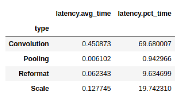
We often want to group information. For example, you may want to know the total latency consumed by each layer type:
# Print the latency of each layer type
plan.df.groupby(["type"]).sum()[["latency.avg_time"]]
Pandas mixes well with other libraries such as dtale, a convenient library for viewing and analyzing dataframes, and Plotly, a graphing library with interactive plots. Both libraries are integrated with the sample TREx notebooks, but there are many user-friendly alternatives such as qgrid, matplotlib, and Seaborn.
There are also convenience APIs that are thin wrappers for Pandas, Plotly, and dtale:
- Plotting data (
plotting.py) - Visualizing an engine graph (
graphing.py) - Interactive notebooks (
interactive.pyandnotebook.py) - Reporting (
report_card.pyandcompare_engines.py)
Finally, the linting API (lint.py) uses static analysis to flag performance hazards, akin to a software linter. Ideally, the layer linters provide expert performance feedback that you can act on to improve your engine’s performance. For example, if you are using suboptimal convolution input shapes or suboptimal placement of quantization layers. The linting feature is in an early development state and NVIDIA plans to improve it.
TREx also comes with a couple of tutorial notebooks and two workflow notebooks: one for analyzing a single engine and another for comparing two or more engines.
With the TREx API you can code new ways to explore, extract, and display TensorRT engines, which you can share with the community.
Example TREx walkthrough
Now that you know how TREx operates, here’s an example that shows TREx in action.
In this example, you create an optimized TensorRT engine of a quantized ResNet18 PyTorch model, profile it, and finally inspect the engine plan using TREx. ] You then adjust the model, based on your learnings, to improve its performance. The code for this example is available in the TREx GitHub repository.
Start by exporting the PyTorch ResNet model to an ONNX format. Use the NVIDIA PyTorch Quantization Toolkit for adding quantization layers in the model, but you don’t perform calibration and fine-tuning as you are concentrating on performance, not accuracy.
In a real use case, you should follow the full quantization-aware training (QAT) recipe. The QAT Toolkit automatically inserts fake-quantization operations into the Torch model. These operations are exported as the QuantizeLinear and DequantizeLinear ONNX operators:
import torch
import torchvision.models as models
# For QAT
from pytorch_quantization import quant_modules
quant_modules.initialize()
from pytorch_quantization import nn as quant_nn
quant_nn.TensorQuantizer.use_fb_fake_quant = True

resnet = models.resnet18(pretrained=True).eval()
# Export to ONNX, with dynamic batch-size
with torch.no_grad():
    input = torch.randn(1, 3, 224, 224)
    torch.onnx.export(
        resnet, input, "/tmp/resnet/resnet-qat.onnx",
    	  input_names=["input.1"],
    	  opset_version=13,
    	  dynamic_axes={"input.1": {0: "batch_size"}})=
Next, use the TREx utility process_engine.py script to do the following:
- Build an engine from the ONNX model.
- Create an engine-plan JSON file.
- Profile the engine execution and store the results in a profiling JSON file. You also record the timing results in a timing JSON file.
python3 <path-to-trex>/utils/process_engine.py /tmp/resnet/resnet-qat.onnx /tmp/resnet/qat int8 fp16 shapes=input.1:32x3x224x224
The script process_engine.py uses trtexec to do the heavy lifting. You can transparently pass arguments to trtexec from the process_engine.py command line by simply listing them without the -- prefix.
In the example, the arguments int8, fp16, and shapes=input.1:32x3x224x224 are forwarded to trtexec, instructing it to optimize for FP16 and INT8 precisions and set the input batch-size to 32. The first script parameter is the input ONNX file (/tmp/resnet/resnet-qat.onnx), and the second parameter (/tmp/resnet/qat) points to the directory to contain the generated JSON files.
You are now ready to examine the optimized engine plan, so go to TREx Engine Report Card notebook. I won’t go through the entire notebook in this post, just a few cells useful for this example.
The first cell sets the engine file and creates a trex.EnginePlan instance from the various JSON files:
engine_name = "/tmp/resnet/qat/resnet-qat.onnx.engine"
plan = EnginePlan(      f"{engine_name}.graph.json",
  f"{engine_name}.profile.json",
  f"{engine_name}.profile.metadata.json")
The next cell creates a visualization of the engine’s data-dependency graph, which is most useful to understanding the transformation of the original network to an engine. TensorRT executes the engine as a topologically sorted layer list, and not as a parallelizable graph.
The default rendering format is SVG, which is searchable, stays sharp at different scales, and supports hover-text for providing additional information without taking up a lot of space.
graph = to_dot(plan, layer_type_formatter)
svg_name = render_dot(graph, engine_name, 'svg')
The function creates an SVG file and prints its name. Rendering inside the notebook is cumbersome even for small networks and you can open the SVG file in a separate browser window for rendering.
The TREx graphing API is configurable, allowing for various coloring and formatting, and the available formatters are packed with information. With the default formatter, for example, layers are colored according to their operation and are labeled by name, type, and profiled latency. Tensors are depicted as edges connecting the layers and are colored according to their precision and labeled with their shape and memory layout information.
In the generated ResNet QAT engine graph (Figure 3), you see some FP32 tensors (in red). Investigate further because you want to have as many layers as possible executing using INT8 precision. Using INT8 data and compute precision increases throughput and lowers latency and power.
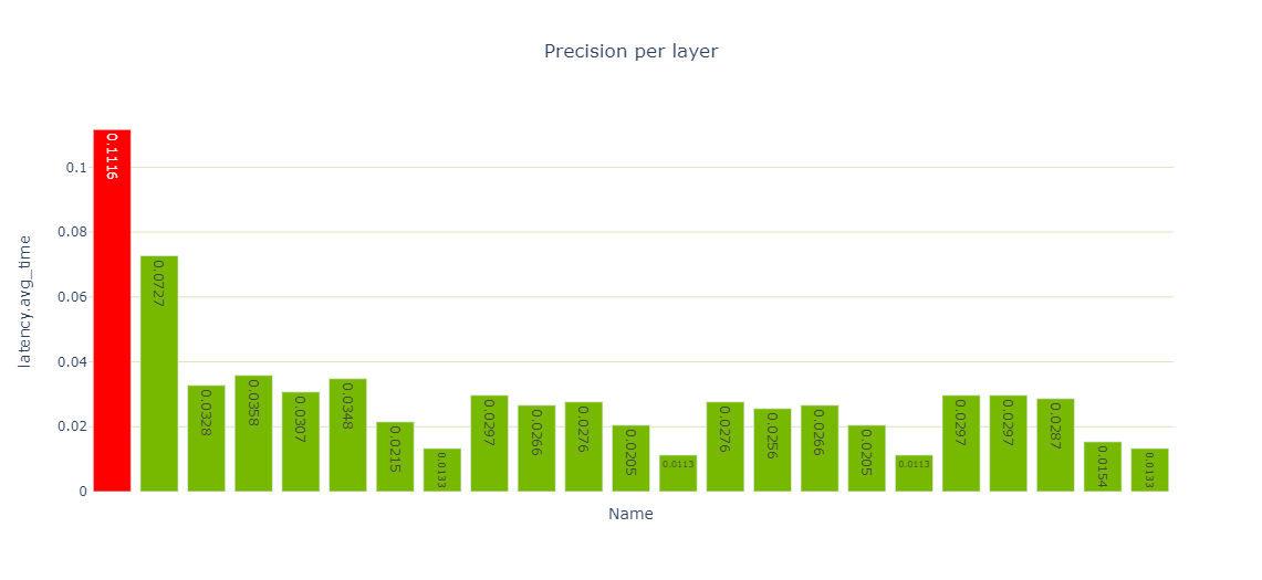
The Performance cell provides various views of performance data, and specifically the precision-per-layer view (Figure 4) shows several layers computing using FP32 and FP16.
report_card_perf_overview(plan)
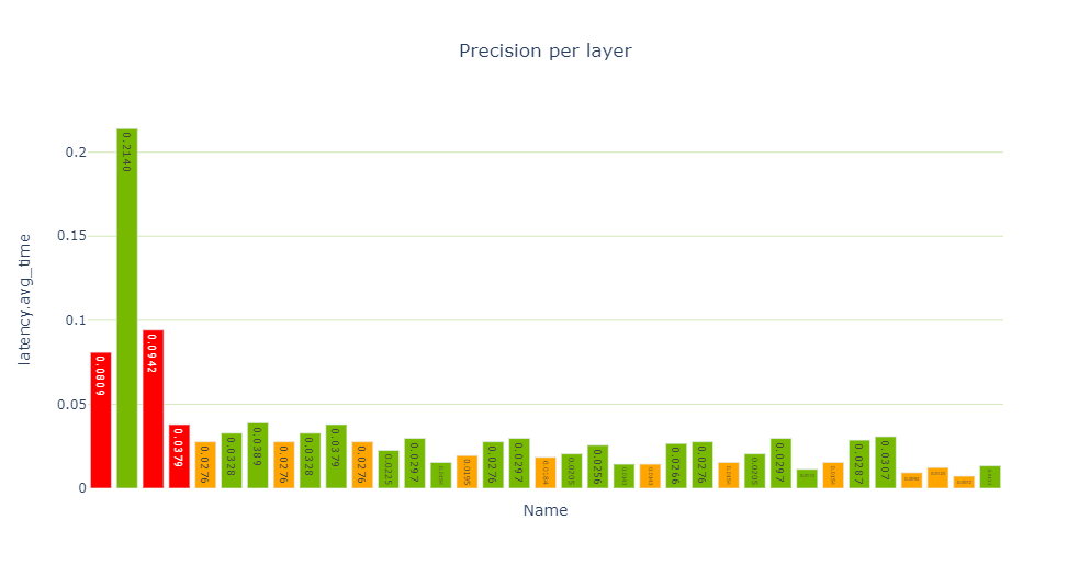
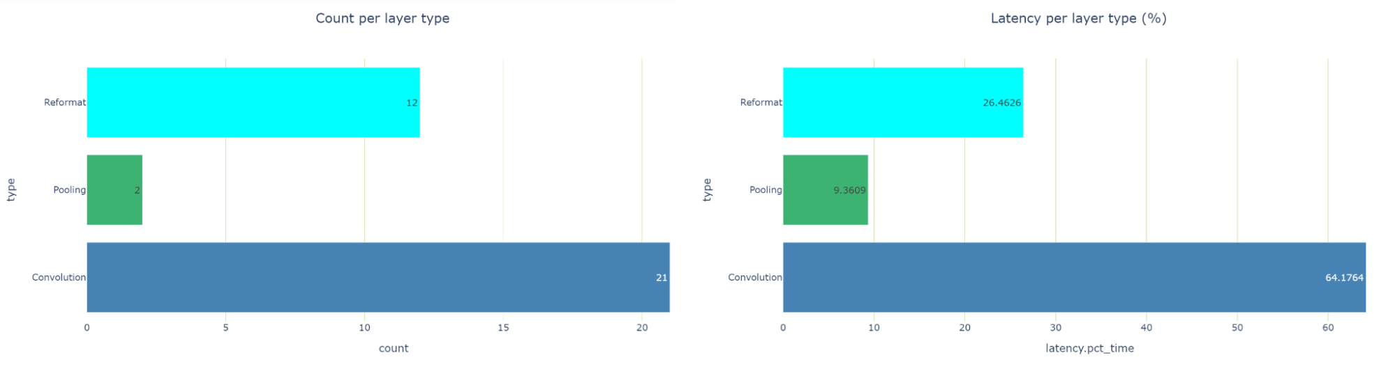
When examining the latency-per-layer-type view, there are 12 reformatting nodes that account for about 26.5% of the runtime. That’s quite a lot. Reformatting nodes are inserted in the engine graph during optimization, but they are also inserted to convert precisions. Each reformat layer has an origin attribute describing the reason for its existence.
If you see too many precision conversions, you should see if there’s something you can do to reduce these conversions. In TensorRT 8.2, you see scale layers, instead of reformatting layers for Q/DQ operations. This is due to the different graph optimization strategies used in TensorRT 8.2 and 8.4.
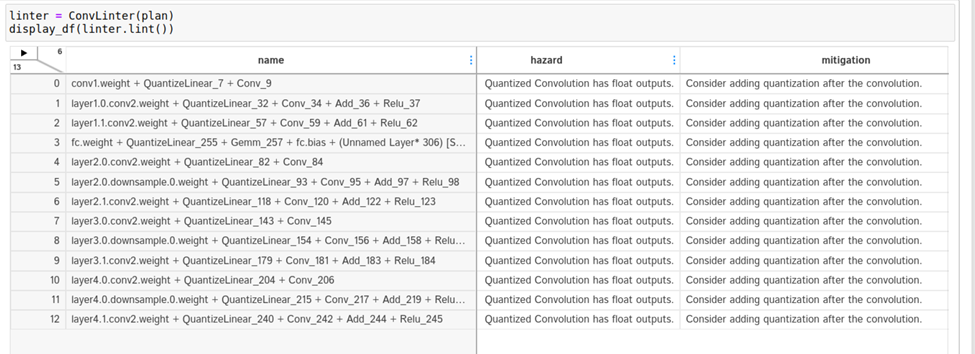
To dig deeper, turn to the engine linting API available in the linting cells. You see that both the Convolution and Q/DQ linters flag some potential problems.
The Convolution linter flags 13 convolutions having INT8 inputs and FP32 outputs. Ideally, you want convolutions to output INT8 data if they are followed by INT8 precision layers. The linter suggests adding a quantization operation following the convolution. Why are the outputs of these convolutions not quantized?
Take a closer look. To look up a convolution in the engine graph, copy the name of the convolution from the linter table and search for it in the graph SVG browser tab. It turns out that these convolutions are involved in residual-add operations.
After consulting Q/DQ Layer-Placement Recommendations, you might conclude that you must add Q/DQ layers to the residual-connections in the PyTorch model. Unfortunately, the QAT Toolkit cannot perform this automatically and you must manually intervene in the PyTorch model code. For more information, see the example in the TensorRT QAT Toolkit (resnet.py).
The following code example shows the BasicBlock.forward method, with the new quantization code highlighted in yellow.
def forward(self, x: Tensor) -> Tensor:
    identity = x
    out = self.conv1(x)
    out = self.bn1(out)
    out = self.relu(out)
    out = self.conv2(out)
    out = self.bn2(out)
    if self.downsample is not None:
        identity = self.downsample(x)

    if self._quantize:
        out += self.residual_quantizer(identity)
    else:
        out += identity
    out = self.relu(out)

    return out
After you change the PyTorch code, you must regenerate the model and iterate again through the notebook cells using the revised model. You’re now down to three reformatting layers consuming about 20.5% of the total latency (down from 26.5%), and most of the layers now execute in INT8 precision.
The remaining FP32 layers surround the global average pooling (GAP) layer at the end of the network. Modify the model again to quantize the GAP layer.
def _forward_impl(self, x: Tensor) -> Tensor:
        # See note [TorchScript super()]
        x = self.conv1(x)
        x = self.bn1(x)
        x = self.relu(x)
        x = self.maxpool(x)

        x = self.layer1(x)
        x = self.layer2(x)
        x = self.layer3(x)
        x = self.layer4(x)

        if self._quantize_gap:
            x = self.gap_quantizer(x)
        x = self.avgpool(x)
        x = torch.flatten(x, 1)
        x = self.fc(x)

        return x
Iterate one final time through the notebook cells using the new model. Now you have only a single reformatting layer and all other layers are executing in INT8. Nailed it!
Now that you are done optimizing, you can use the Engine Comparison notebook to compare the two engines. This notebook is useful not only when you are actively optimizing your network’s performance as you’re doing here, but also in the following situations:
- When you want to compare engines built for different GPU HW platforms or different TensorRT versions.
- When you want to assess how layers’ performance scales across different batch sizes.
- To understand if accuracy disagreement between engines is due to different TensorRT layer precision choices.
The Engine Comparison notebook provides both tabular and graphical views to compare engines and both are applicable, depending on the level of details that you need. Figure 8 shows the stacked latencies of five engines that we’ve built for the PyTorch ResNet18 model. For brevity, I didn’t discuss creating the FP32 and FP16 engines, but these are available in the TREx GitHub repository.
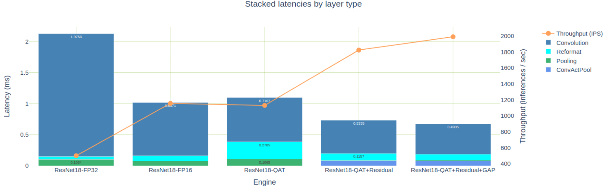
The engine optimized for FP16 precision is about 2x faster than the FP32 engine, but it is also faster than our first attempt at an INT8 QAT engine. As I analyzed earlier, this is due to the many INT8 convolutions that output FP16 data and then require reformat layers to quantize explicitly back to INT8.
If you concentrate only on the three QAT engines optimized in this post, you can see how you eliminated 11 FP16 engine layers when you added Q/DQ to the residual connections. You eliminated another two FP32 layers when you quantized the GAP layer.

You can also look at how the optimizations affected the latencies of the three engines (Figure 10).
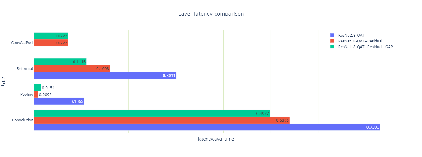
You may notice a couple of odd-looking, pooling-layer, latency results: the total pooling latency drops 10x when you quantize the residual connection, and then goes up 70% when you quantize the GAP layer.
Both results are counterintuitive so look at them more closely. There are two pooling layers, a large one after the first convolution, and another tiny one before the last convolution. After you quantized the residual-connections, the first pooling and convolution layers could execute using the output in INT8 precision. They are fused with the sandwiched ReLU into a ConvActPool layer, but this fusion is not supported for floating-point types.
Why did the GAP layer increase in latency when it was quantized? Well, the activation size of this layer is small and each INT8 input coefficient is converted to FP32 for averaging using high precision. Finally, the result is converted back to INT8.
The layer’s data size is also small and resides in the fast L2 cache, and thus the extra precision-conversion computation is relatively expensive. Nonetheless, because you could get rid of the two reformat layers surrounding the GAP layer, the total engine latency (which is what you really care about) is reduced.
Summary
In this post, I introduced the TensorRT Engine Explorer, briefly reviewed its APIs and features, and walked through an example showing how TREx can help when optimizing the performance of a TensorRT engine. TREx is available in TensorRT’s GitHub repository, under the experimental tools directory.
I encourage you to try the APIs and to build new workflows beyond the two workflow notebooks.
