An End-to-End Blueprint for Accelerating Customer Churn Modeling and Prediction-Part 1

Editor’s Note: Get notified and be the first to download our real-world blueprint once it’s available.

If you want to solve a particular kind of business problem with machine learning, you’ll likely have no trouble finding a tutorial showing you how to extract features and train a model. However, building machine learning systems isn’t just about training models or even about finding the best features; if you want a blueprint for a real system or want to see how to address more of the data science workflow, many tutorials leave the hard parts as an exercise for the reader.

Over several installments, we’ll be building a blueprint for predicting customer churn — that is, identifying customers who are likely to cancel subscriptions. We’ll pay special attention to parts of the process that are underserved by most data science tutorials, such as analytic processing and federation of structured data, integrating enterprise data engineering pipelines with machine learning, and production model serving. We’ll also show you how to accelerate each stage of this workflow with NVIDIA GPUs.

In this installment, we’ll level-set by introducing a typical end-to-end machine learning workflow and the overall architecture for our churn prediction solution. We’ll then examine the first part of our solution: a data engineering pipeline that federates and integrates structured transactional data and prepares it for further processing by a data scientist, with a special focus on ensuring our pipeline can take advantage of the RAPIDS Accelerator for Apache Spark. In future installments, we’ll dive deep into other parts of the problem related to data science and DevOps workflows: feature extraction, model training, deployment, and accelerated inference.

Machine learning workflows and the customer churn problem

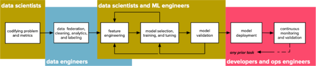
Ten years ago, a “data scientist” was a practitioner whose role combined domain expertise with elements of analytics, applied statistics, machine learning, software engineering, and even infrastructure operations and was responsible for data storytelling and end-to-end machine learning solutions. Definitions evolve, and today a typical data scientist is more specialized and only focuses on parts of the classic machine learning workflow: characterizing data, finding patterns, and training models. The other parts of the classic workflow are still important, but the practitioners who are responsible for them may have different names for their roles, such as data engineer, application developer, machine learning engineer, or MLOps engineer. The figure below shows such a workflow and the personas involved at each stage, borrowing concrete terminology from an IEEE Software article.

Alt. text: a schematic depiction of a machine learning workflow, showing how data scientists begin by codifying the problem under consideration; data engineers federate, clean, and label data; data scientists engage in a modeling workflow involving feature extraction, model training, and model validation; and, finally, developers and ops engineers put the model and learning pipeline into production and set up continuous monitoring infrastructure.) — *Figure 1. A typical machine-learning workflow, with the personas involved at each stage*.

Our system for churn modeling and prediction will focus on data federation, data analytics, feature engineering, model training, and model deployment, and will consist of three applications that work together: an analytic application that integrates structured data from a data warehouse, a feature extraction, and model training application that takes flat training data and generates a trained model, and an inference service that takes information about a customer and predicts whether or not that customer will churn.

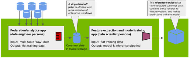
Alt. text: an architecture diagram showing databases feeding in to an analytics application, which outputs data to a database table that is ultimately consumed by a feature extraction and model training application. The output of the latter informs a production inference service. — *Figure 2. Overall system architecture for churn modeling and detection*.

We’ll also be using this system to demonstrate how and when you can use RAPIDS and the RAPIDS Accelerator for Apache Spark to accelerate workloads with GPUs. Let’s examine the analytics application now, starting with the dataset we’ll use.

Synthesizing data at scale

Since real-world customer retention data isn’t typically freely available, we’ll begin with a synthetic dataset that approximates a telecommunications company’s customer records. This data set is open-source and there are several excellent open-source tutorials using it to demonstrate machine learning techniques. However, many data science and ML tutorials do not treat two important aspects of contemporary enterprise data pipelines:

They operate at minimal scale (in the case of this example, the source dataset is roughly 7,000 records). This allows users to experiment with modeling techniques quickly but doesn’t provide an opportunity to engage many of the challenges of processing larger datasets and training models at a realistic scale.
They begin with denormalized, wide-form data as it might appear on a data scientist’s desk, not with multiple tables from a data warehouse that needs to be aggregated and federated in order to integrate all of the data we have about each given customer.

Our goal in this blueprint is to show an interesting churn modeling problem at meaningful scale and to show the query workloads that a data engineer might develop to prepare wide-form data for a data scientist. In order to do that, we’ll need more data and normalized data:

We’re going to augment the initial dataset by generating multiple synthetic customers that are essentially identical to each customer in the initial dataset, and
For each row in the augmented dataset, we’re going to generate records in multiple tables as they might exist in an enterprise data warehouse. One table of customer information will become five tables containing observations about a customer’s behavior.

Generating wide tables from customer account data

Now that we have the five normalized tables about customer accounts and activity, we can simulate the data engineering pipeline that would prepare a flat, wide table for a data scientist to process and model. Essentially, this consists of multiple joins, aggregations, and transformations, including;

Rolling up billing event counts (to calculate account tenure) and billing amounts (to calculate lifetime account value),
Identifying whether a customer is a senior citizen or not based on their birthdate, and
Reconstructing wide-form account features (services and billing data) from long-form tables

We’ve implemented this pipeline with a Python application that uses Apache Spark.

Improving analytics performance

Remember that our overall data science workflow isn’t a waterfall; it’s a cycle. Since we might want to change the nature of our analytics job in order to meet new downstream requirements (or to fix bugs), we might have to rerun the job at any time. Since humans will often be waiting for the result of analytics jobs or ad hoc analytic queries, we want these jobs to be as fast as possible to make the most of human time and attention. Here are some techniques we used while developing this application; you can use these as well to improve the performance of your Spark query workloads.

Inspect

Use the tools that Spark provides to help understand what your job is actually doing: look at the web UI to determine where your application is spending time and ensure that it is adequately using all of the resources it has reserved. Inspect the query plans generated by DataFrame.explain to ensure that a seemingly-simple query doesn’t imply a pathological execution plan.

Upgrade and optimize

There are often engineering costs involved with validating applications against new versions of frameworks, and enterprises can be conservative about upgrading Spark. But if you can run your application on Spark 3.0 or greater, you’ll benefit from improved performance relative to the 2.x series, especially if you enable Adaptive Query Execution, which will use runtime statistics to dynamically choose better partition sizes, more efficient join types, and limit the impact of data skew.

Accelerate and understand

Once you’re on Spark 3.0, consider using the RAPIDS Accelerator for Apache Spark, which has the potential to dramatically speed up DataFrame-based Spark applications. However, like any advanced optimization, you’ll want to make sure you understand how to make the most of it. Here are some concrete tips:

Some applications are better candidates for GPU acceleration than others. The RAPIDS accelerator plugin works by translating query plans to run on columnar data in GPU memory and thus it cannot accelerate code that processes RDDs or operates on data one row at a time. Applications that spend a lot of time using RDDs as well as DataFrames, or that use complex user-defined functions, will not see the maximum possible speedup.
Start with the suggested configuration in RAPIDS Accelerator for Apache Spark Tuning Guide. Remember that if you want to use more than one GPU on a given system, you’ll need to run more than one Spark worker process on that system — each JVM will only be able to access one GPU.
Once you’re up and running with the GPU, make sure to use the tools available to you again. This means revisiting the Spark web UI and DataFrame.explain — but this time, look out for query plan nodes that don’t run on the GPU. You can also configure the plugin to tell you why certain parts of your application did or did not run on the GPU by setting the property spark.rapids.sql.explain to ALL or NOT_ON_GPU; if you set this option, make sure you have access to console output from your application.

Diving in a bit to understand how the application was executing on the GPU made it possible to unlock additional performance. When we looked at the query graph, we were able to determine that two parts of the query were unable to run on the GPU as we had configured the application: aggregating total lifetime account values and determining whether or not a customer with a given birthdate is a senior citizen. These two issues caused parts of the query to execute on CPU and parts to execute on the GPU, meaning that there were more transfers of data between the CPU and the GPU than strictly necessary; as it turned out, only the first one seriously impacted performance.

Fortunately, the fix was very simple: the RAPIDS Accelerator plugin will not perform aggregates on floating-point values by default because the roundoff behavior may be different from a CPU execution due to parallel execution.

However, we can set the property spark.rapids.sql.variableFloatAgg.enabled to True and accelerate these operations as well. (If we were processing real money, we’d use a more precise number format, but for modeling behavior, floating-point values are a great choice.) By making this change, we were able to improve our performance by 2x relative to an already-fast GPU execution.

Next steps

See the documentation for the RAPIDS Accelerator for Apache Spark for instructions to get started with GPU acceleration in your own workloads. Future installments of this series will cover more details of our blueprint, including feature extraction, model training, and production deployments.