Molecular dynamics (MD) simulations are a powerful tool in computational chemistry and materials science, and they’re essential for studying chemical reactions, material properties, and biological interactions at a microscopic level. However, their complexity and computational requirements often necessitate advanced techniques such as machine learning interatomic potentials (MLIPs) to achieve scalability, efficiency, and accuracy.
Integrating PyTorch-based MLIPs into the LAMMPS MD package through the ML-IAP-Kokkos interface enables fast and scalable simulation of atomic systems for chemistry and materials science research.
This interface was developed through a collaborative effort between NVIDIA, Los Alamos National Lab, and Sandia National Lab scientists. It was designed to simplify the process of interfacing community models for external developers, allowing them to seamlessly connect MLIPs with LAMMPS enabling scalable MD simulations.
The ML-IAP-Kokkos interface supports message-passing MLIP models, utilizing LAMMPS’s built-in communication capabilities to facilitate efficient data transfer between GPUs—something that’s crucial for enabling large-scale simulations that leverage the computational power of multiple GPUs. The interface uses Cython to bridge Python and C++/Kokkos LAMMPS, ensuring end-to-end GPU acceleration, optimizing the overall simulation workflow.
We’ll walk you through how to connect your own PyTorch models for scalable LAMMPS simulation, step-by-step. Let’s get started.
Preparing your tools and environment
- Experience with LAMMPS or other MD simulation tools.
- Experience using Python, familiarity with PyTorch and machine learning models (Cython a plus).
- Optional: for additional acceleration, cuEquivariance supported models and NVIDIA GPUs.
Building your own ML-IAP-Kokkos Interface
Step 1: Setting up the environment
Ensure you have all necessary software installed:
- LAMMPS built with Kokkos, MPI, and ML-IAP
- Python with PyTorch
- Trained PyTorch MLIP model (optionally with cuEquivariance support)
Step 2: Install LAMMPS with ML-IAP-Kokkos/Python support
Download and install LAMMPS (September 2025 release or later) with Kokkos, MPI, ML-IAP and Python support.
Installing LAMMPS with Python support also installs the lammps module in your Python environment.
For convenience, we have prepared a container with a precompiled LAMMPS.
Step 3: Develop ML-IAP-Kokkos interface for preferred model
When using the ML-IAP-Kokkos interface, LAMMPS will call the Python interpreter during the simulation, executing your native Python model and providing all Python features without having to compile your model. This requires a working Python environment with access to your model’s classes.
To connect your model with LAMMPS, you need to implement the abstract class MLIAPUnified from LAMMPS as defined in `mliap_unified_abc.py`. Specifically, you need to make the compute_forces function infer pairwise forces and energies using the data passed to it from LAMMPS (the class will also require compute_gradients and compute_descriptors functions, but these can be empty as they will not be used in this setup).
Starting with a simple example to understand the data that LAMMPS passes to your class, we create a class that prints some information:
from lammps.mliap.mliap_unified_abc import MLIAPUnified
import torch


class MLIAPMod(MLIAPUnified):
    def __init__(
        self,
        element_types = None,
    ):
        super().__init__()
        self.ndescriptors = 1
        self.element_types = element_types
        self.rcutfac = 1.0 # Half of radial cutoff
        self.nparams = 1


    def compute_forces(self, data):
        print(f"Total atoms: {data.ntotal}, Local atoms: {data.nlocal}")
        print(f"Atom indices: {data.iatoms}, Atom types: {data.elems}")
        print(f"Neighbor pairs: {data.npairs}")
        print(f"Pair indices and displacement vectors: ")
        print("\n".join([f"   ({i}, {j}), {r}" for i,j,r in zip(data.pair_i, data.pair_j, data.rij)]))
Note that the __init__ function specifies the element types our model can handle and (half) the neighbor list’s cutoff radius. These parameters are required by LAMMPS in model setup.
We save our model object with the PyTorch save function:
mymodel = MLIAPMod(["H", "C", "O"])
torch.save(mymodel, "my_model.pt")
This creates the file my_model.pt, a “pickled” Python object, which LAMMPS can load. In a real scenario this would contain the weights of our model but here it’s a serialization of our class. (In the latest versions of PyTorch, loading a class is disabled by default as a security protection since the class contains arbitrary Python code. Setting the environment variable TORCH_FORCE_NO_WEIGHTS_ONLY_LOAD=1 allows loading the class. Use only trusted *.pt files).
For testing, we will define a system of a single CO2 molecule in the file sample.pos:
#The mandatory first line is a comment and skipped!
3 atoms
2 atom types

0.0 100.0 xlo xhi
0.0 100.0 ylo yhi
0.0 100.0 zlo zhi

Masses

1 12.0
2 16.0

Atoms

1 2 1.0 10.0 10.0
2 1 2.0 10.0 10.0
3 1 -0.1 10.0 10.0
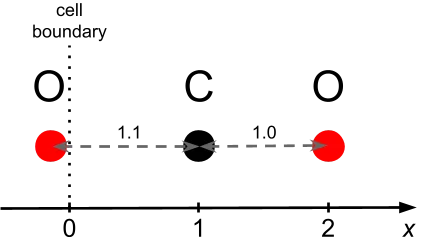
The molecule consists of one carbon atom and two oxygen atoms arranged linearly along the X-axis, with the carbon located at x = 1.0 Å and the oxygen atoms at x = -0.1 Å and x = 2.0 Å, respectively. This minimal configuration allows us to clearly observe how LAMMPS handles local versus ghost atoms, pair interactions, and periodic boundary conditions—key elements for understanding the data flow in the interface.
Figure 1 illustrates the atomic positions and their relationship to the simulation cell boundaries.
The following LAMMPS input sample.in loads the position file, loads our potential, and runs a single MD step:
units           metal
atom_style      atomic
atom_modify     map array
boundary p p p
read_data   sample.pos


# Load the ML-IAP model
pair_style      mliap unified my_model.pt 0
pair_coeff      * * C O


dump dump0 all custom 1 output.xyz id type x y z fx fy fz
run 0
Using the pair style mliap, the “unified” keyword directs LAMMPS to use the Python interface, followed by the model file to load, and finally the value 0, which affects the neighbor list (see documentation for details).
We specify the subset of elements we are interested in (C and O) and their mapping to the indices in the positions file.
We run LAMMPS with Kokkos on one GPU with the command:
lmp -k on g 1 -sf kk -pk kokkos newton on neigh half -in sample.in
And look at this relevant part of the output:
Total atoms: 6, Local atoms: 3
Atom indices: [0 1 2], Atom types: [2 1 1 2 1 1]
Neighbor pairs: 4
Pair indices and displacement vectors:
   (0, 5), [-1.1  0.   0. ]
   (0, 1), [1. 0. 0.]
   (1, 0), [-1.  0.  0.]
   (2, 3), [1.1 0.  0. ]
Comparing this with our class, we understand the data structure:
- Atoms are divided into two categories: physical atoms, ranging from
[0, nlocal), which need to be updated; and ghost atoms ranging from[nlocal, ntotal), which are either periodic copies or physical atoms from another processor/GPU. - There are three local atoms (
nlocal) and three ghost atoms for a total of six (ntotal). iatomslists the indices of local atoms (the first nlocal).elemslists the atomic species of all atoms.npairsis the number of pairs within the cutoff that involve at least one local atom.
Note that pairs (i, j) and (j, i) are reported separately: here we have four pairs corresponding to the two (C, O) bonds in either direction.
We can access the (i, j) indices of each pair and the relative displacement via pair_i, pair_j, and rij.
Note that indices greater than or equal to nlocal refer to ghost atoms (e.g. 3 is the periodic ghost of 0, 5 is the periodic ghost of 2).
To implement a simple potential, imagine a model that computes some “node features” on local atoms and updates the energy based on neighbor features and bond lengths, a typical setup for MLIPs. For simplicity, take all features to be 1 and the radial function to be the atomic distance (in an actual implementation, these would be more complex objects computed by our model).
A (partial) implementation of this potential might be:
   def compute_forces(self, data):
        rij = torch.as_tensor(data.rij)
        rij.requires_grad_()
        features = torch.zeros((data.ntotal,1)).cuda()
        for i in range(data.nlocal):
            features[i,0] = 1.0
        Ei = torch.zeros(data.nlocal).cuda()


        # Message passing step (j → i)
        for r,i,j in zip(rij, torch.as_tensor(data.pair_i), torch.as_tensor(data.pair_j)):
            Ei[i] += features[j,0] * torch.norm(r)

        # Compute total energy and forces
        Etotal = torch.sum(Ei)
        Fij = torch.autograd.grad(Etotal, rij)[0]


        # Copying total energy and forces
        data.energy = Etotal
        data.update_pair_forces_gpu(Fij)
Some details to notice in this code:
- All quantities passed between the ML-IAP and LAMMPS are fp64 and on device, although type-casting and host<->device movement is permitted in the model.
- Total energy is updated directly in our model.
- We compute forces through the autograd function with respect to rij, i.e. forces are computed “per bond” and not “per atom.” Potentials that compute atomic forces directly must be recast in this form.
We update the forces in LAMMPS through the function update_pair_forces_gpu, passing the fp64 GPU tensor of shape (npairs, 3).
We test this code on our small CO2 molecule.
For reference, we compute energies and forces by hand with only two pairs and two distances (1 and 1.1), the total energy should be 4.2, with each pair contributing 1 to the force, yielding a force of 2 in opposite directions for the carbons, with 0 force on the oxygen.
However, running this code we obtain a total energy of 2 (as seen in stdout) and force 2 (as seen in output.xyz) on one carbon and the oxygen. It’s clear that the problem is the presence of ghost atoms; their features are not updated on the real atoms so that only the (0, 1) bond contributes to the total energy and forces.
In this simplified case, we could initialize the ghosts to 1, but in a real scenario, this might be a more complex function of the environment. In that case, we use the message passing hooks built into ML-IAP-Kokkos to update the ghost features to the value of their corresponding real counterparts. This takes care of ghost particles coming from periodic boundary conditions and those residing on an entirely different GPU.
Two routines are provided to help this initialization process: forward_exchange, which sets ghost atoms from their physical counterparts; and reverse_exchange, which sums contributions made to ghost atoms back to their physical counterparts.
Step 4: Implementing message passing support for ML-IAP-Kokkos
Updating our model to use the message passing step (see code below), we call forward_exchange, which takes two tensors of shape (ntotal, feat_size) and sets features[0,nlocal) to new_features[0,ntotal), handling local copying and MPI messaging. The feat_size, 1 here, is the vector width of the feature. This function creates a copy of features with ghost values set from their physical counterparts.
 def compute_forces(self, data):
        rij = torch.as_tensor(data.rij)
        rij.requires_grad_()
        features = torch.zeros((data.ntotal,1)).cuda()
        for i in range(data.nlocal):
            features[i,0] = 1.0
        Ei = torch.zeros(data.nlocal).cuda()

        # Update of the features
        new_features = torch.empty_like(features)
        data.forward_exchange(features, new_features, 1)
        features = new_features


        # Local message passing step
        for r,i,j in zip(rij, torch.as_tensor(data.pair_i), torch.as_tensor(data.pair_j)):
            Ei[i] += features[j,0] * torch.norm(r)

        # Compute total energy and forces
        Etotal = torch.sum(Ei)
        Fij = torch.autograd.grad(Etotal, rij)[0]


        # Copying total energy and forces
        data.energy = Etotal
        data.update_pair_forces_gpu(Fij)
Running this code again, we now obtain the correct energy and forces. However, on multiple GPUs, the force calculation would not work correctly as the gradients are not computed across different devices.
To fix this, we need to define and register the gradient of LAMMPS_MP.forward() with PyTorch. The gradient of forward_exchange is provided via reverse_exchange. After calling reverse_exchange, gradients are confined to real atoms and zeroed on all ghost atoms.
Here is a simple implementation of the complete message passing:
import torch
class LAMMPS_MP(torch.autograd.Function):
    @staticmethod
    def forward(ctx, *args):
        feats, data = args  # unpack
        ctx.vec_len = feats.shape[-1]
        ctx.data = data
        out = torch.empty_like(feats)
        data.forward_exchange(feats, out, ctx.vec_len)
        return out


    @staticmethod
    def backward(ctx, *grad_outputs):
        (grad,) = grad_outputs  # unpack
        gout = torch.empty_like(grad)
        ctx.data.reverse_exchange(grad, gout, ctx.vec_len)
        return gout, None
With this new class, the final version of our plugin becomes:
 def compute_forces(self, data):
        rij = torch.as_tensor(data.rij)
        rij.requires_grad_()
        features = torch.zeros((data.ntotal,1)).cuda()
        for i in range(data.nlocal):
            features[i,0] = 1.0
        Ei = torch.zeros(data.nlocal).cuda()

        # Update of the features
        features = LAMMPS_MP().apply(features, data)


        # Local message passing step
        for r,i,j in zip(rij, torch.as_tensor(data.pair_i), torch.as_tensor(data.pair_j)):
            Ei[i] += features[j,0] * torch.norm(r)


        # Compute total energy and forces
        Etotal = torch.sum(Ei)
        Fij = torch.autograd.grad(Etotal, rij)[0]


        # Copying total energy and forces
        data.energy = Etotal
        data.update_pair_forces_gpu(Fij)
We now have access to proper multi-GPU message passing that correctly supports autograd.
This same structure should work independently of message passing MLIP models.
Calling LAMMPS_MP before any message passing ensures that features remain synchronized and the model works correctly. Optimization may exist, however, where some communication steps may be skipped. Since LAMMPS collects ghosts before calling the ML-IAP and since LAMMPS propagates forces on ghosts to other ranks afterwards, the first forward exchange and last reverse exchange in a multi-layer MLIP can often be skipped.
As mentioned, the force calculation requires the computation of energy gradients with respect to bonds. Additionally, passing all terms to LAMMPS allows LAMMPS to tally the contributions for the computation of stresses; stresses don’t need to be computed by the plugin.
Evaluating performance with the HIPPYNN model
To demonstrate the performance improvements that the message passing hooks enable, we benchmarked LAMMPS running with HIPPYNN (Chigaev 2023) models in multiple series of weak scaling tests on one to 512 NVIDIA H100 GPUs with models comprised of h=1 to h=4 interaction layers in the MLIP with and without the communication hooks. We use a simple lattice of aluminum atoms as a performance test, keeping the number of atoms to approximately 203 atoms per GPU.
The models were trained on the dataset from the paper Automated discovery of a robust interatomic potential for aluminum following the example multi-interaction layer training script in HIPPYNN. For simulation correctness, where r is the interaction radius of one MLIAP layer, we use a ghost cutoff length r+epsilon with the hooks enabled and hr+epsilon with ghost-ghost pairs enabled in the neighbor list when the hooks are disabled.
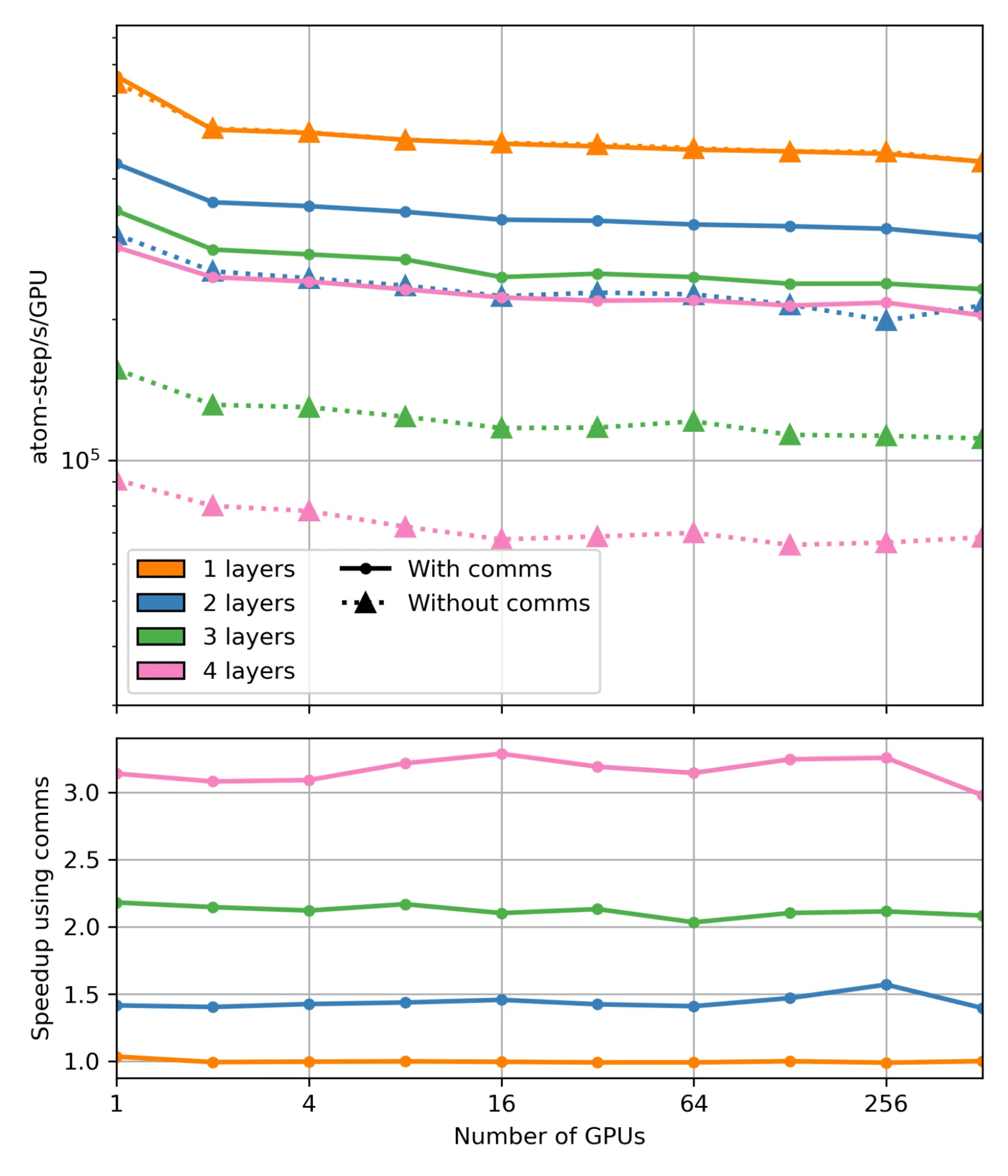
The speedup from using the communication hooks shown in the figure above is directly attributable to the reduction in ghost atoms. The percentage of real atoms to total atoms (real plus ghost) with one, two, three, and four layers of ghost atoms is 54%, 38%, 26%, and 18%, respectively. With hooks enabled, we can use one radius of ghosts and thus 54% real atoms for all cases. This leads to a 1.4x, 2.1x, and 3x reduction in total atoms for two, three, and four layers, respectively (for one layer, the hooks are non-operative), directly corresponding to the observed speedups.
Comparing results using MACE integration
As one further demonstration, we benchmark LAMMPS simulations using the popular MLIP MACE comparing the original MACE pairstyle in LAMMPS, which utilizes libtorch in C++ to load model weights, to a cuEquivariance-based MACE plugin using the MLIAP-Kokkos interface. cuEquivariance is an NVIDIA Python library for accelerating geometric neural networks.
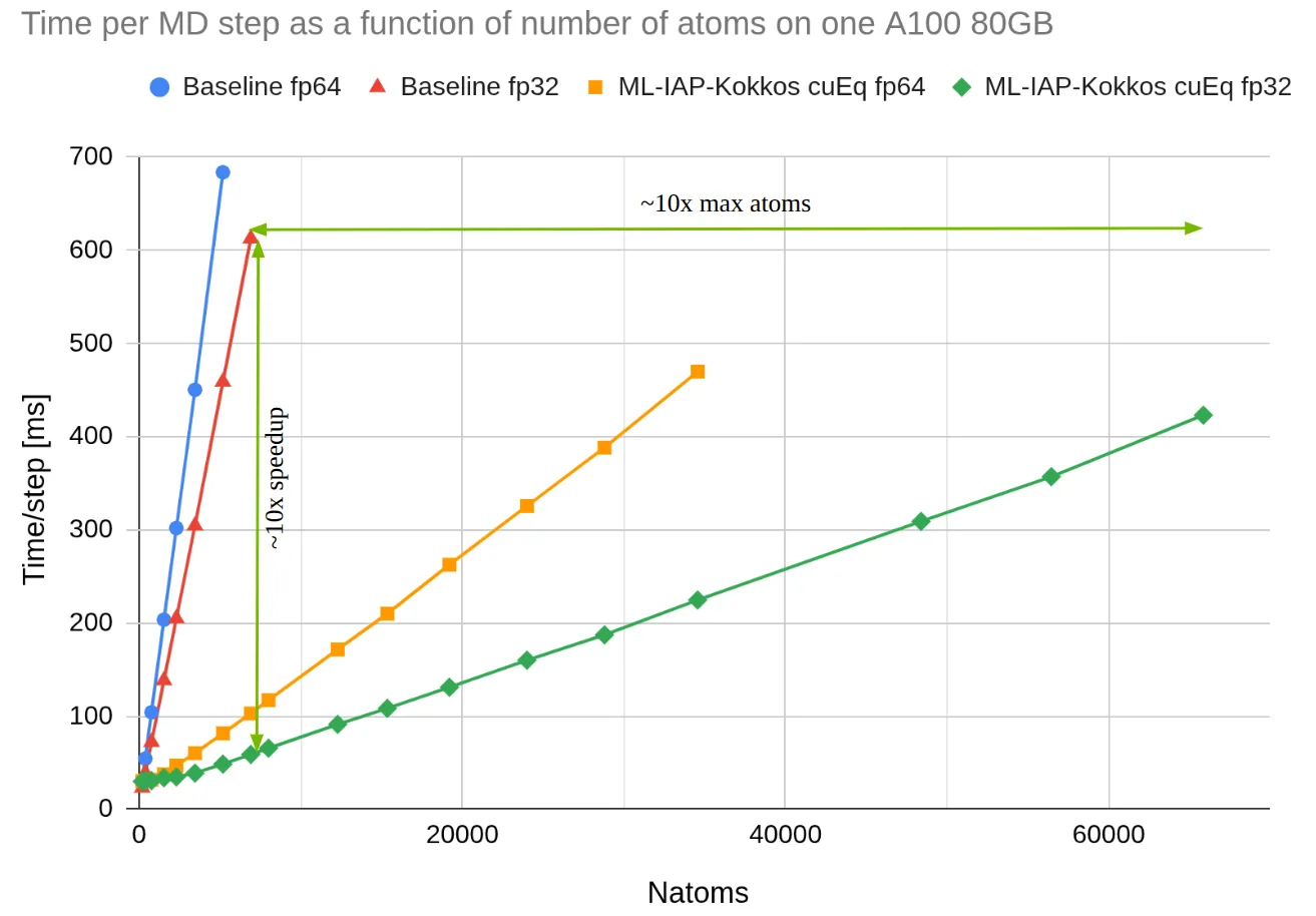
For this benchmark, we simulate increasingly larger boxes of water until GPU memory is exhausted using the “medium” version of the MACE-OFF23 potential on a single A100 GPU with 80GB of memory with fp32 and fp64 models. The speed of the original MACE pairstyle is shown for comparison. The new plugin is far faster and more memory efficient. This speedup is attributable to model acceleration with cuEquivariance and the message passing improvements in the MLIAP-Kokkos interface. CuEquivariance accelerated MLIPs can be seamlessly used in LAMMPS when passing through the ML-IAP-Kokkos interface.
Conclusion
The LAMMPS ML-IAP-Kokkos interface is currently the most important tool enabling multi-GPU, multi-node MD simulations using MLIPs. It allows the simulation of extremely large systems with high efficiency, bridging the gap between modern ML-based force fields and high-performance computing infrastructures.
By integrating PyTorch-based MLIPs with LAMMPS via the ML-IAP-Kokkos interface, developers can achieve scalable and efficient MD simulations. This tutorial outlines the steps necessary to set up and execute simulations and highlights the benefits of GPU acceleration and message-passing capabilities in LAMMPS. The benchmark results further emphasize the interface’s potential for large-scale simulations, making it a valuable tool for researchers and developers in the field.
Ready to accelerate your simulations? Try the tutorial today and share your results with the community. Subscribe to NVIDIA news and follow NVIDIA AI on LinkedIn, X, Discord, and YouTube.