Traditional healthcare systems have large amounts of patient data in the form of physiological signals, medical records, provider notes, and comments. The biggest challenges involved in developing digital health applications are analyzing the vast amounts of data available, deriving actionable insights, and developing solutions that can run on embedded devices.
Engineers and data scientists working with biomedical datasets often run into challenges while developing such end-to-end solutions because they must manually integrate their application code, integrate with necessary toolchains to deploy, and in many cases rewrite code to run the application on target hardware. If the algorithm does not yield the expected results, they must debug the underlying case, which can be time-consuming.
This post discusses how data scientists and engineers can prototype AI-based digital health algorithms for biomedical applications using NVIDIA GPUs and deploy such algorithms on embedded IoT and edge AI platforms like NVIDIA Jetson. You can also use MathWorks GPU Coder to deploy the prediction pipeline on Jetson.
The solution goal is to train a classifier to distinguish between Arrhythmia (ARR), Congestive Heart Failure (CHF), and Normal Sinus Rhythm (NSR). This tutorial uses ECG data obtained from three groups, or classes:
- People with cardiac arrhythmia
- People with congestive heart failure
- People with normal sinus rhythms
The example uses 162 ECG recordings from three PhysioNet databases and each recording has 65536 samples:
- MIT-BIH Arrhythmia Database: 96 recordings
- BIDMC Congestive Heart Failure Database: 30 recordings
- MIT-BIH Normal Sinus Rhythm Database:36 recordings
To run this example, you need the following resources:
- MATLAB
- Wavelet Toolbox
- Signal Processing Toolbox
- Parallel Computing Toolbox
- GPU Coder
- MATLAB Coder
- GPU Coder Support Package for NVIDIA GPUs
Request a product trial or send us an email at medical@mathworks.com.
Overall workflow for developing AI-based digital health applications
There are many approaches for developing a predictive model for ECG signals. The focus of this post is to explore a simplified workflow that combines advancements in signal processing and leverages the large body of work already done in developing convolutional neural network (CNNs) and deep learning architectures for ECG signal classification. Figure 1 shows the overall workflow.
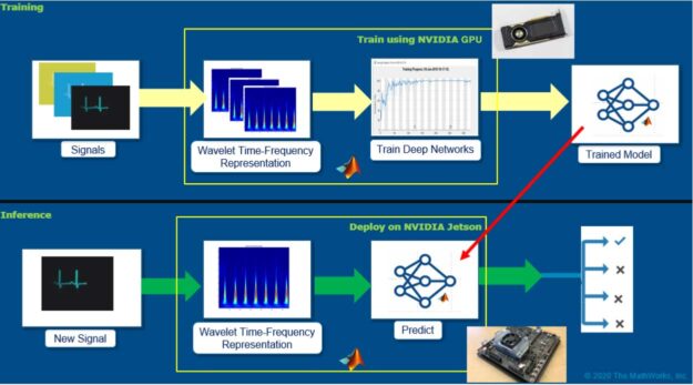
The main idea here is to generate time-frequency representations from ECG signals and save those representations as images. A time-frequency representation of ECG captures how the spectral components evolve as a function of time. These images can be subsequently used to train convolutional neural networks (CNNs). The CNNs can extract features from the patterns present in the images (the time-frequency representations of ECG signals) and can build a model to discriminate the ECG signals belonging to various classes.
After you develop the model, you can then deploy the pipeline: time-frequency representations and the trained model on embedded hardware such as Jetson to perform inference on new signals using GPU Coder. GPU Coder automatically generates optimized CUDA code from MATLAB algorithms.
Speeding up time-frequency representations using NVIDIA Quadro RTX 6000
Here’s how to generate time-frequency representations from ECG records. Although there are several methods in MATLAB to generate time-frequency representations from signals, we highly recommend using continuous wavelet transform (CWT) for its simplicity and ability to generate sharp time-frequency representations from signals. The time-frequency representation thus generated is also referred to as scalogram.
The CWT is obtained by windowing the signal with a wavelet that is scaled and shifted in time. The wavelet oscillates and can be complex-valued. The scaling and shifting operations are applied to a prototype wavelet. The scaling used in the CWT both shrinks and stretches the prototype wavelet:
- Shrinking the prototype wavelet yields short-duration, high-frequency wavelets that are good at detecting transient events.
- Stretching the prototype wavelet yields long duration, low-frequency wavelets that are good at isolating long-duration, low-frequency events.
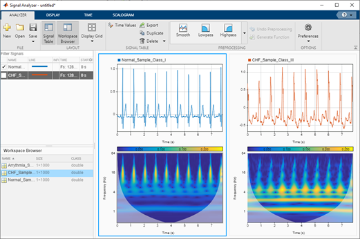
Having such sharp time-frequency representations can be useful as deep networks or CNNs are good at extracting features from such representations and building a predictive model. Another benefit of using sharp time-frequency representations is that it enables you to build models to capture the subtle variations that can in turn help discriminate between many classes of signals, even if the signals look similar.
To speed up the scalogram generation process, you can run MATLAB functions on GPUs if you convert the input variables to the type gpuArray. You can then use the gather function to retrieve the output data from the GPU. For speeding up the process of generating the scalograms, use the function cwtfilterbank to create the wavelet filter bank one time and then use the wt method of cwtfilterbank for generating the time-frequency representations.
We used NVIDIA Quadro RTX 6000 to compute the scalograms and were able to achieve a speed-up of ~6.5x. The CPU used was Intel Xeon CPU E5-1650 v4 @3.60 GHz with 64-GB RAM.
For more information, see the cwt and cwtfilterbank function reference.
load('ECGData.mat');  % Data file downloaded from git

useGPU = true;
tic;
X = helperTimeScalogramConversion(ECGData, useGPU);
Tgpu = toc;

useGPU = false;
tic;
X = helperTimeScalogramConversion(ECGData, useGPU);
Tcpu = toc;


function X = helperTimeScalogramConversion(ECGData, useGPU)

data = ECGData.Data;
[Nsamples,signalLength] = size(data);

fb = cwtfilterbank('SignalLength',signalLength,'VoicesPerOctave',12);
X = zeros(numel(fb.scales), signalLength, Nsamples);

r = size(data,1);

if useGPU
    data = single(gpuArray(data));
else
    data = single(data);
end

for ii = 1:r
    cfs = abs(fb.wt(data(ii,:)));
    X(:,:,ii) = gather(cfs);

end
end
Using GPU: false
Number of signals: 162
-------------------------------------
Total execution time Tcpu =   67.32 s
-------------------------------------
Using GPU: true
Number of signals: 162
-------------------------------------
Total execution time Tgpu =   10.28 s
-------------------------------------
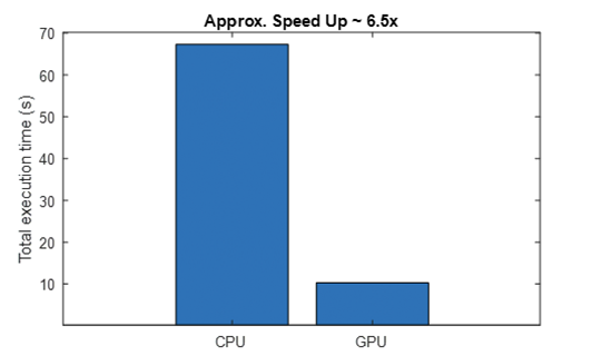
From the command line output and the generated plot, you can see that using GPUs results in a significant speedup (6.5x). This becomes useful when you have multiple signals. Later, you might see that the ability to generate scalograms on GPU would be a key enabler for developing the application on the Jetson platform.
Training CNNs to classify ECG signals using Quadro RTX 6000
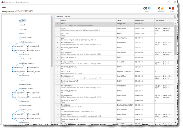
Now that you have the time-frequency images of the ECG signals, you can apply transfer learning on a pretrained, deep learning network to build your classifier. For this example, retrain SqueezeNet, which is an 18 layer-deep network trained on more than a million images. This is a lightweight network with lower memory footprint and better inference speeds, characteristics that are ideal for embedded deployment. The network originally trained on 1000 image classes, but you can fine-tune the network using the three ECG image classes datasets to build your new classifier.
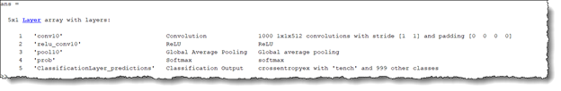
First, inspect the original network, which contains 18 layers including convolution, ReLU, and fire block (a combination of the convolution and ReLU layers). Figure 4 shows a code example of the layers displayed in MATLAB by running the following command:
analyzeNetwork(squeezeNet)
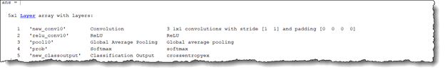
To retrain SqueezeNet to classify the three classes of ECG signals, replace the last conv10 layer with a new convolutional layer with the number of filters equal to the number of ECG classes. Also, replace the classification layer with a new one without class labels.
sqz = squeezenet;
lgraph = layerGraph(sqz);
lgraph.Layers(end-4:end)
numClasses = 3; % Number of ECG signal classes new_conv10_WeightLearnRateFactor = 1;
new_conv10_BiasLearnRateFactor = 1;
newConvLayer = convolution2dLayer(1,numClasses,...
        'Name','new_conv10',...
        'WeightLearnRateFactor',new_conv10_WeightLearnRateFactor,...
        'BiasLearnRateFactor',new_conv10_BiasLearnRateFactor);
lgraph = replaceLayer(lgraph,'conv10',newConvLayer);
newClassLayer = classificationLayer('Name','new_classoutput');
lgraph = replaceLayer(lgraph,'ClassificationLayer_predictions',newClassLayer);
lgraph.Layers(end-4:end)
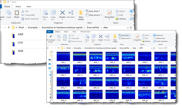
For deep learning training, you can now load the images of the ECG scalogram data saved as JPEGs in the respective folders ARR, CHF, and NSR (Figure 7). For more information about the scripts used to save the scalogram data into JPEG images, see Classify Time-Series using Wavelet Analysis and Deep Learning.
The imageDatastore function is used to create an image datastore for these images with the label names derived from the respective folder names, and is divided into training (70%), validation (10%) and test (20%) subsets. You also associated a readFcn object with the datastore to automatically resize the images to 227x227x3 and meet the SqueezeNet input image requirements.
readFcn = @(imagefilename)imresize(imread(imagefilename), [227 227]);
imds = imageDatastore('../data', 'LabelSource', 'foldernames', ...
                     'IncludeSubFolder', true, 'readFcn', readFcn);
[imgsTrain, imgsValidation, imgsTest ]  = splitEachLabel(imds, 0.7, 0.1, 0.2);
The next step is to define the training hyperparameters and pass the network for training. If you have a GPU installed, MATLAB automatically scales the training on the GPU. To train without a GPU (not recommended), use multiple GPUs or scale the training on the cloud. You can do so by adjusting the ExecutionEnvironment parameter in trainingOptions.
options = trainingOptions('sgdm',...
    'MiniBatchSize',15,...
    'MaxEpochs',20,...
    'InitialLearnRate',1e-4,...
    'ValidationData',imgsValidation,...
    'ValidationFrequency',10,...
    'Momentum',0.9,...
    'ExecutionEnvironment', 'auto');

trainedModel = trainNetwork(imgsTrain,lgraph,options);
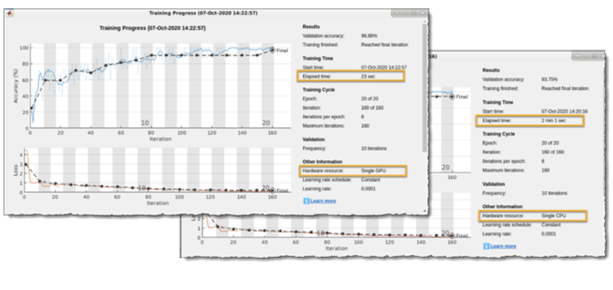
We trained this network using NVIDIA Quadro RTX 6000. Figure 8 shows that it took only 23 seconds to train the network. This is significantly faster (~6x) when compared to training time on CPU. MATLAB automatically uses the CUDA and cuDNN libraries to accelerate the training when using GPUs. However, it is worth mentioning that we were working with only 162 time-frequency images and as such, the overall training time was quite smaller. The training time performance of GPU compared to CPU scales up as the amount of training data increases.
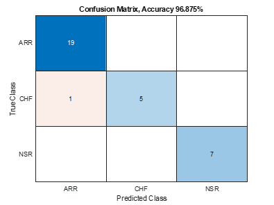
Now that you have a trained model, you can verify the accuracy by inferencing the test image dataset, which the new model has never seen before. We did train an accurate model with >95% classification accuracy having only one misclassification.
predictedLabels = classify(trainedModel, imgsTest);
accuracy = sum(predictedLabels == imgsTest.Labels) / numel(predictedLabels);
confusionchart(imgsTest.Labels, predictedLabels)
title("Confusion Matrix, Accuracy " + accuracy*100 + "%")
Deploy digital health IoT applications on Jetson
Now that you have trained and built your AI application, it is time for deployment. The NVIDIA Jetson platform offers small, power-efficient system-on-modules with high-compute performance and cloud-native capabilities, making it an excellent candidate for deploying digital health IoT applications. You can deploy the whole pipeline (time-frequency generation and SqueezeNet prediction) on the Jetson platform so that it can run the algorithms independently.
In this example, read in live ECG signals from an IO module, convert the signal to a time-frequency image using CWT, and finally pass the image through the trained, deep learning network to provide an inference. All these steps are executed in real time, such that there is no delay between acquiring the ECG signals and getting the inference results.
Using GPU Coder, MATLAB provides an automated pathway on converting the various signal processing, wavelet analysis, image processing, and deep learning algorithms into optimized CUDA code that can be directly put into production on the Jetson platform.
As a first step, package the AI application into MATLAB functions as it would run in the deployed version. As shown in the code example, the function model_predict_ecg takes in an ECG signal of 65536 samples as input, passes it to function cwt_ecg_jetson_ex to convert it into a time-frequency image, passes it through the trained deep learning network, and finally provides the probability scores of all the different ECG classes as the output.
%% MATLAB functions for deployment
function PredClassProb = model_predict_ecg(TimeSeriesSignal)

    coder.gpu.kernelfun();

    % parameters
    ModFile = 'ecg_model.mat'; % file that saves neural network
    ImgSize = [227 227]; % input image size for the ML model

    % sanity check signal is a row vector of correct length
    assert(isequal(size(TimeSeriesSignal), [1 65536]))

    %% cwt transformation for the signal
    im = cwt_ecg_jetson_ex(TimeSeriesSignal, ImgSize);

    %% model prediction
    persistent model;
    if isempty(model)
        model = coder.loadDeepLearningNetwork(ModFile, 'mynet');
    end

    PredClassProb = predict(model, im);

end

function im = cwt_ecg_jetson_ex(TimeSeriesSignal, ImgSize)

coder.gpu.kernelfun();

%% Create scalogram
cfs = cwt(TimeSeriesSignal, 'morse', 1, 'VoicesPerOctave', 12);
cfs = abs(cfs);

%% Image generation

% Load the jet colormap generated and saved earlier using the commands:
% >> cmapj128 = jet(128); save(‘cmapj128.mat’, ‘cmapj128’);

cmapj128 = coder.load('cmapj128');
imx = ind2rgb_custom_ecg_jetson_ex(round(255*rescale(cfs))+1,cmapj128.cmapj128);

% Resize to proper size and convert to uint8 data type
im = im2uint8(imresize(imx, ImgSize));

end

function out = ind2rgb_custom_ecg_jetson_ex(a, cm)

   indexedImage = a;

   % Make sure that indexedImage is in the range from 1 to number of colormap
   % entries
   numColormapEntries = size(cm,1);
   indexedImage = max(1, min(indexedImage, numColormapEntries) );

   height = size(indexedImage, 1);
   width = size(indexedImage, 2);

   rgb = coder.nullcopy(zeros(height,width,3));
   rgb(1:height, 1:width, 1) = reshape(cm(indexedImage, 1), [height width]);
   rgb(1:height, 1:width, 2) = reshape(cm(indexedImage, 2), [height width]);
   rgb(1:height, 1:width, 3) = reshape(cm(indexedImage, 3), [height width]);

   out = rgb;

end
Now that you have your functions set up, connect to the Jetson platform from MATLAB. The GPU Coder Support Package for NVIDIA GPUs supports the following developer kits:
- NVIDIA Jetson TK1
- Jetson TX1
- Jetson TX2
- Jetson AGX Xavier
- Jetson Xavier NX
- Jetson Nano
It also supports the NVIDIA DRIVE platform. Here is the code example to connect to the Jetson Nano platform and set up the configuration parameters for generating CUDA code from the earlier functions.
hwobj = jetson('gpucoder-nano-2','username','password');
cfg = coder.gpuConfig('exe');
cfg.Hardware = coder.hardware('NVIDIA Jetson');
cfg.Hardware.BuildDir = '~/remoteBuildDir';
cfg.DeepLearningConfig = coder.DeepLearningConfig('cudnn');
cfg.CustomSource = fullfile('main_ecg_jetson_ex.cu');
The code example specified including the custom source file main_ecg_jetson_ex.cu as an argument in the code generation. This was done to specify the input/output pipeline for testing the deployed algorithm on the Jetson platform. You first generated the sample main.cu template for this application by selecting the GenerateExampleMain property of coder.gpuConfig object to GenerateCodeOnly. Following this, you modified the template main.cu file to include reading the sample ECG signal data from a text file, signalData.txt, and writing the results of the algorithm to another text file, predClassProb.txt. The modified main.cu file was saved as main_ecg_jetson_ex.cu and is provided for reference.
//
// File: main_ecg_jetson_ex.cu
//
//***********************************************************************
// Include Files
#include "rt_nonfinite.h"
#include "model_predict_ecg.h"
#include "main_ecg_jetson_ex.h"
#include "model_predict_ecg_terminate.h"
#include "model_predict_ecg_initialize.h"
#include <stdio.h>
#include <stdlib.h>
#include <time.h>

// Function Definitions

/* Read data from a file*/
int readData_real32_T(const char * const file_in, real32_T data[65536])
{
  FILE* fp1 = fopen(file_in, "r");
  if (fp1 == 0)
  {
    printf("ERROR: Unable to read data from %s\n", file_in);
    exit(0);
  }
  for(int i=0; i<65536; i++)
  {
      fscanf(fp1, "%f", &data[i]);
  }
  fclose(fp1);
  return 0;
}

/* Write data to a file*/
int writeData_real32_T(const char * const file_out, real32_T data[3])
{
  FILE* fp1 = fopen(file_out, "w");
  if (fp1 == 0)
  {
    printf("ERROR: Unable to write data to %s\n", file_out);
    exit(0);
  }
  for(int i=0; i<3; i++)
  {
    fprintf(fp1, "%f\n", data[i]);
  }
  fclose(fp1);
  return 0;
}

// model predict function
static void main_model_predict_ecg(const char * const file_in, const char * const file_out)
{
  real32_T PredClassProb[3];
  //  real_T b[65536];
  real32_T b[65536];

  // readData_real_T(file_in, b);
  readData_real32_T(file_in, b);

  model_predict_ecg(b, PredClassProb);

  writeData_real32_T(file_out, PredClassProb);

}

// main function
int32_T main(int32_T argc, const char * const argv[])
{
  const char * const file_out = "predClassProb.txt";
  // Initialize the application.
  model_predict_ecg_initialize();

  // Run prediction function
  main_model_predict_ecg(argv[1], file_out); // argv[1] = file_in

  // Terminate the application.
  model_predict_ecg_terminate();
  return 0;
}

//
// End of file
//
The code generation command is then executed to generate and build the CUDA code and deploy it on the Jetson device. This command generates the compiled model_predict_ecg.elf file and puts it on the Jetson build directory path specified in the code generation configuration parameter, cfg.Hardware.BuildDir.
inputSignal = coder.newtype('single', [1 65536], [0 0]);
codegen model_predict_ecg.m -args {inputSignal} – config cfg -report
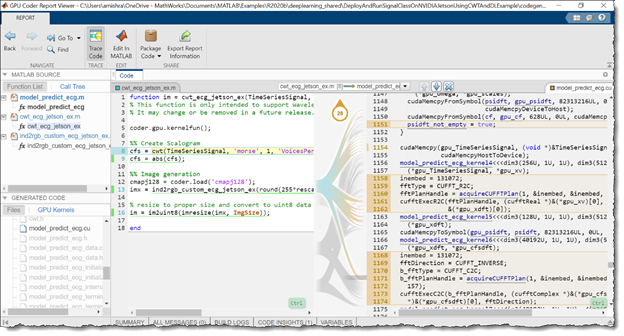
First, inspect the following autogenerated code. More than 30 CUDA kernels were automatically created for performing time-frequency image conversion and deep learning prediction steps. GPU Coder automatically invokes the optimized NVIDIA CUDA cuDNN libraries for deep learning and the cuBLAS, cuFFT, and cuSolver libraries for other matrix computations. Figure 10 shows the generated report GUI, which can be used to inspect the autogenerated CUDA files and trace the generated CUDA code back to the respective MATLAB functions.
Now that you’ve generated the code, test the performance of the algorithm on the Jetson. You can either run the generated executable directly from the Jetson or use the MATLAB interface to execute the application directly from MATLAB. In this example, you write a sample ECG data file, signalData.txt, to the workspace directory of the Jetson and execute your compiled application on the Linux terminal of the board.
sampleIndx = 113; % Chose any ECG record from the ECGData struct for testing
signal_data = ECGData.Data(sampleIndx, :);
ECGType = ECGData.Labels(sampleIndx);

fid = fopen('signalData.txt','w');
for i = 1:length(signal_data)
   fprintf(fid,'%f\n',signal_data(i));
end
fclose(fid);

% Copy the text file to the workspace directory on the Jetson board
hw.putFile('signalData.txt', hwobj.workspaceDir)
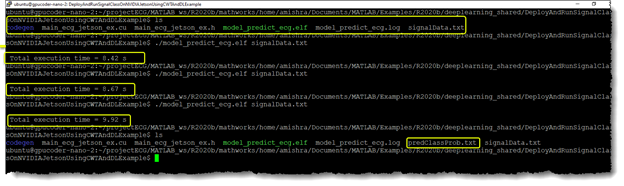
Open the Jetson terminal. Inside the workspace, you find the copied signalData.txt file along with a compiled model_predict_ecg.elf and folder codegen. When you executed the application multiple times to log the speed of execution, the application output created the predClassProb.txt output file, which contains the probability scores for classifying the input signal by the application.
The output text file can be loaded back in MATLAB. Compare the inference results from Jetson with inference results from MATLAB running on CPU. You see that the test signal was a normal sinus rhythm, and both Jetson as well as MATLAB had the highest probability score for the NSR class.
% Fetch the result file from Jetson
resultFile = 'predClassProb.txt';
resultFile_hw = fullfile(hwobj.workspaceDir,resultFile);
hwobj.getFile(resultFile_hw)
PredClassProb = readmatrix(resultFile);
PredTableJetson = array2table(PredClassProb(:)','VariableNames',matlab.lang.makeValidName(PredCat));

% Execute the function in MALTAB
ModPredProb = model_predict_ecg(signal_data);
PredTableMATLAB = array2table(ModPredProb(:)','VariableNames',matlab.lang.makeValidName(PredCat));

% Display the probability scores from Jetson
disp(PredTableJetson)

      ARR         CHF        NSR
    ________    _______    _______

    0.026817    0.17381    0.79937


% Display the probability scores from MATLAB
disp(PredTableMATLAB)

      ARR         CHF        NSR
    ________    _______    _______

    0.026863    0.17401    0.79913
Conclusion
In this post, we covered how you can easily develop AI-based digital health applications and deploy these algorithms on embedded IoT and edge AI platforms, such as NVIDIA Jetson. This workflow simplifies the process of developing the AI applications for physiological signals like ECG signals using transfer learning techniques. It provides a good starting point for developing such algorithms.
For more information, see the following resources: