
Medical image segmentation is a hot topic in the deep learning community. Proof of that is the number of challenges, competitions, and research projects being conducted in this area, which only rises year over year. Among all the different approaches to this problem, U-Net has become the backbone of many of the top-performing solutions for both 2D and 3D segmentation tasks. This is due to its simplicity, versatility, and effectiveness.
When practitioners are confronted with a new segmentation task, the first step commonly is to use an existent implementation of U-Net as a backbone. But with the arrival of TensorFlow 2.0, there is a lack of available solutions that you can use off-the-shelf. How can you effectively transition models to TensorFlow 2.0 to take advantage of the new features, while still maintaining top hardware performance and ensuring state-of-the-art accuracy?
U-Net for medical image segmentation
U-Net was first introduced by Olaf Ronneberger, Philip Fischer, and Thomas Brox in the paper, U-Net: Convolutional Networks for Biomedical Image Segmentation. U-Net allows for the seamless segmentation of 2D images with high accuracy and performance. It can be adapted to solve many different segmentation problems.
Figure 2 shows the construction of the U-Net model and its different components. U-Net is composed of a contractive and an expanding path, which aims to build a bottleneck in its centermost part through a combination of convolution and pooling operations. After this bottleneck, the image is reconstructed through a combination of convolutions and upsampling. Skip connections are added with the goal of helping the backward flow of gradients to improve the training.

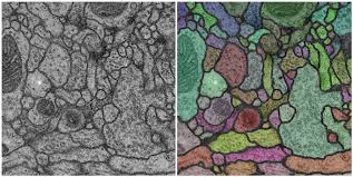
The task where U-Net excels is often referred to as semantic segmentation, and it entails labeling each pixel in an image with its corresponding class reflecting what is being represented. Because you are doing this for each pixel in an image, this task is commonly referred to as dense prediction.
In the case of semantic segmentation, the expected outcome of the prediction is a high-resolution image, typically of the same dimensions as the image being fed to the network, in which every pixel is labeled to the corresponding class. Generalizing broadly, semantic segmentation is just a form of pixel-wise, multi-class classification.
Even though U-Net was primarily designed for semantic segmentation, it is not uncommon to see U-Net-based networks achieving very good results in tasks such as object detection or instance segmentation.
Migrating to TensorFlow 2.0 with performance in mind
Usually the first step when working with deep learning models is to establish a baseline with which you’re comfortable. In the NVIDIA Deep Learning Examples Github repository, you can find the implementation of the most popular deep learning models. These implementations cover almost every domain and framework and provide extensive benchmarks ensuring optimal accuracy and performance. Because of that, they are an optimal starting point for you, whether you’re a practitioner or researcher.
Among these implementations, you can find U-Net, available in TensorFlow 1.x and TensorFlow 2.0. But what are the steps to follow to migrate to the newest version of TensorFlow?
A new way to run models
One of the most noticeable changes in this new version of TensorFlow is the switch between using sessions to function calls. Until now, you would specify the inputs and the function to be called and would expect back the outputs of the model. The execution of the graph then was performed inside a session.run call, as shown in the following code example:
TensorFlow 1.X
outputs = session.run(f(placeholder), feed_dict={placeholder: input})
TensorFlow 2.0
outputs = f(input)
This is possible due to eager execution being enabled by default in TensorFlow 2.0. This changes the way that you interact with TensorFlow, as eager execution is an imperative programming environment that evaluates operations immediately. It offers benefits such as a more intuitive interface, easier debugging, natural control flow, but at the expense of worse performance. It is typically recommended for research and experimentation.
AutoGraph
To achieve production-grade performance in models using TensorFlow 2.0, you must use AutoGraph (AG). This Tensorflow 2.0 feature lets you write TensorFlow graph code using natural Python syntax by using the decorator @tf.function, as shown in the following code example:
@tf.function
def train_step(features, targets, optimizer):
With tf.GradientTape() as tape:
        predictions = model(features)
        loss = loss_fn(predictions, targets)
    vars = model.trainable_variables
gradients = tape.gradient(loss, vars)
optimizer = apply_gradients(zip(gradients, vars))
Even though AG still has limitations, the performance improvement that it delivers is noticeable. For more information about how to achieve better performance with tf.function and AG, see the TensorFlow 2.0 Guide.
Maximizing Tensor Core usage
Mixed precision is the combined use of different numerical precision in a computational method. Mixed precision training offers significant computational speedup by performing operations in half-precision format while storing minimal information in single-precision to retain as much information as possible in critical parts of the network.
After the introduction of Tensor Cores in the Volta and Turing architectures, you can experience significant training speedups by switching to mixed precision: up to 3x overall speedup on the most arithmetically intense model architectures. Using mixed precision training requires two steps:
- Porting the model to use the FP16 data type where appropriate.
- Adding loss scaling to preserve small gradient values.
For more information, see the following resources:
- Mixed Precision Training paper
- Training With Mixed Precision documentation.
- Mixed-Precision Training of Deep Neural Networks post.
- Using TF-AMP from the TensorFlow User Guide.
Enabling automatic mixed precision training
To enable automatic mixed precision (AMP) in TensorFlow 2.0, you must apply the following changes to the code.
Set Keras mixed precision policy:
tf.keras.mixed_precision.experimental.set_policy('mixed_float16')
Use the loss scaling wrapper on the optimizer. By default, you can select dynamic loss scaling:
optimizer = tf.keras.mixed_precision.experimental.LossScaleOptimizer(optimizer, "dynamic")
Make sure that you’re using the scaled loss to calculate gradients:
loss = loss_fn(predictions, targets)scaled_loss = optimizer.get_scaled_loss(loss)

vars = model.trainable_variables
scaled_gradients = tape.gradient(scaled_loss, vars)
gradients = optimizer.get_unscaled_gradients(scaled_gradients)

optimizer.apply_gradients(zip(gradients, vars))
Enabling Accelerated Linear Algebra
Accelerated Linear Algebra (XLA) is a domain-specific compiler for linear algebra that can accelerate TensorFlow models with potentially no source code changes. The results are improvements in speed and memory usage: most internal benchmarks run ~1.1-1.5x faster after XLA is enabled.
To enable XLA, set up the just-in-time (JIT) graph compilation in your optimizer. You can do this with the following change to your code:
tf.config.optimizer.set_jit(True)
U-Net in TensorFlow 2.0
In the NVIDIA Deep Learning Examples GitHub repository, you can find an implementation of U-Net using TensorFlow 2.0. This implementation contains all the necessary pieces, not only to port U-Net to the new version of Google’s framework, but also to migrate any TensorFlow 1.x trained model using tf.estimator.Estimator.
Besides the necessary changes described earlier related to the performance of the model, follow these steps to make sure that the model is fully compliant with the new API:
- API cleanup
- Data loading
- Model definition
API cleanup
As many API actions have been removed or have changed location in TensorFlow 2.0, the first step is to use the v2 upgrade script to replace deprecated calls with their new equivalents:
tf_upgrade_v2 \
  --intree unet_tf1/ \
  --outtree unet_tf2/ \
  --reportfile report.txt
Even though this conversion script automates most of the process, some changes still have to be made manually, according to the recommendations captured in the report file. For more information, TensorFlow offers the following guide, Automatically upgrade code to TensorFlow 2.
Data loading
The data pipeline used to train the model is the same used for the TensorFlow 1.x implementation. It is implemented using tf.data.Dataset API action. The data pipeline loads an image and transforms it using different data augmentation techniques. For more information, see the data_loader.py script.
Model definition
This new version of TensorFlow encourages you to refactor your code into smaller functions and to modularize different components. One of them is model definition, which can now be performed by subclassing tf.keras.Model:
class Unet(tf.keras.Model):    """ U-Net: Convolutional Networks for Biomedical Image Segmentation
    Source:
        https://arxiv.org/pdf/1505.04597
    """
    def __init__(self):
        super().__init__(self)
        self.input_block = InputBlock(filters=64)
        self.bottleneck = BottleneckBlock(1024)
        self.output_block = OutputBlock(filters=64, n_classes=2)

        self.down_blocks = [DownsampleBlock(filters, idx)
                            for idx, filters in enumerate([128, 256, 512])]

        self.up_blocks = [UpsampleBlock(filters, idx)
                          for idx, filters in enumerate([512, 256, 128])]

    def call(self, x, training=True):
        skip_connections = []
        out, residual = self.input_block(x)
        skip_connections.append(residual)

        for down_block in self.down_blocks:
            out, residual = down_block(out)
            skip_connections.append(residual)

        out = self.bottleneck(out, training)

        for up_block in self.up_blocks:
            out = up_block(out, skip_connections.pop())

        out = self.output_block(out, skip_connections.pop())
        return tf.keras.activations.softmax(out, axis=-1)
Performance results
With the aforementioned changes, run the model to verify the speedup delivered by Tensor Cores on TensorFlow 2.0. There are three different features influencing performance:
- The use of TensorFlow AG
- The use of Accelerated Linear Algebra (XLA)
- The use of automatic mixed precision (AMP) using Tensor Cores
Training performance
Our results were obtained by running in the tensorflow:20.02-tf2-py3 NGC container on NVIDIA DGX-1 with (8x V100 16G) GPUs. Performance numbers (in items/images per second) were averaged over 1000 iterations, excluding the first 200 warm-up steps.
| GPUs | Batch size / GPU | Throughput – FP32 [img/s] | Throughput – mixed precision [img/s] | Throughput speedup (FP32 – mixed precision) |
| 1 | 8 | 17.98 | 51.89 | 2.89 |
| 8 | 8 | 143.08 | 386.15 | 2.70 |
The example model was able to reach a 2.89x speedup measured in images per second using mixed precision in TensorFlow 2.0 for single GPU training, and a 2.7x speedup for multi-GPU training with 8 GPUs, with almost perfect weak scaling factor using mixed precision. For more information, see the steps that we followed.
Figure 3 shows an extra insight into how the different features available in TensorFlow 2.0 influence the performance of the training phase. The most effective way to boost the throughput of the model is by enabling AMP, with all the setups including this feature being among the top-performing ones. When training using mixed precision though, XLA delivers a boost only when you use AG. The combination of AMP, XLA, and AG delivers the best results.

Inference performance
The example results were obtained by running in the tensorflow:20.02-tf2-py3 NGC container on NVIDIA DGX-1 with (1x V100 16G) GPU. Throughput is reported in images per second. Latency is reported in milliseconds per batch.
| Batch size | Throughput – Fp32 Avg [img/s] | Throughput – mixed precision Avg [img/s] | Throughput speedup (FP32 – mixed precision) |
| 8 | 58.66 | 187.65 | 3.19 |
This model can reach a 3.19x speedup using mixed precision in TensorFlow 2.0 on inference. For more information, see the Inference performance benchmark steps.
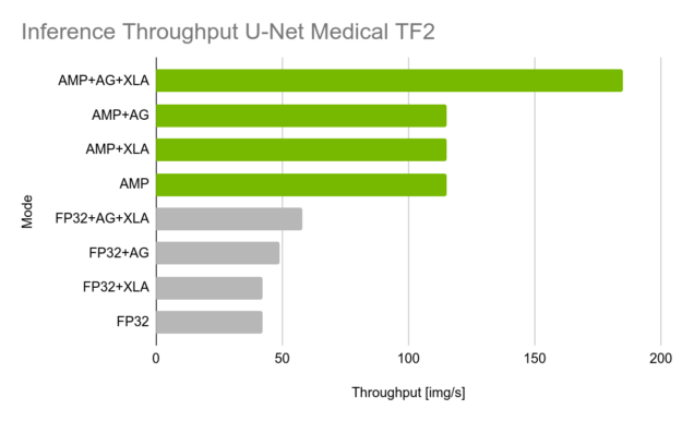
Figure 4 shows an extra insight on how the different features available in TensorFlow 2.0 influence the performance of the inference phase. The most important boost in performance appears when AMP is enabled, as Tensor Cores greatly accelerate the prediction. Because the model is already trained, you can disable eager execution by enabling AG, which delivers an extra boost.
Next steps
You can begin taking advantage of the new features in TensorFlow 2.0 with your NVIDIA GPUs. TensorFlow 2.0 greatly simplifies the process of training a model and it is easier than ever to take advantage of Tensor Cores in the newest version of the framework.
In the Deep Learning Examples repository, you’ll find more than 25 open-source implementations of the most popular deep learning models. They are available in TensorFlow, PyTorch, and MXNet. In these examples are step-by-step guides on how to run these models with state-of-the-art accuracy and record-breaking performance.
All implementations are shipped with instructions about how to perform mixed precision training to accelerate your model using Tensor Cores. We also distribute these models pretrained in the form of checkpoints. These models are fully maintained and include the latest features, such as multi-GPU training, data loading using DALI, and TensorRT deployment.
Stay tuned to and keep an eye out for new models. Do you have any suggestions? Let us know by opening an issue in NVIDIA Deep Learning Examples.
