Building Medical 3D Image Segmentation Using Jupyter Notebooks from the NGC Catalog

The NVIDIA NGC team is hosting a webinar with live Q&A to dive into this Jupyter notebook available from the NGC catalog. Learn how to use these resources to kickstart your AI journey. Register now: NVIDIA NGC Jupyter Notebook Day: Medical Imaging Segmentation.

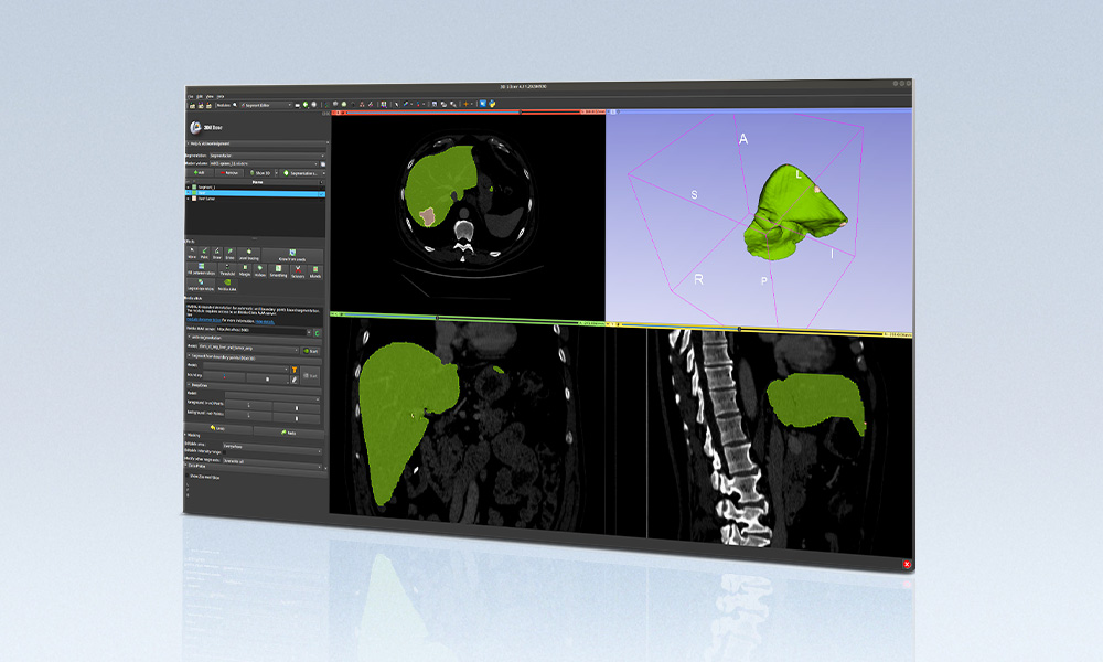
Image segmentation partitions a digital image into multiple segments by changing the representation into something more meaningful and easier to analyze. In the field of medical imaging, image segmentation can be used to help identify organs and anomalies, measure them, classify them, and even uncover diagnostic information. It does this by using data gathered from x-rays, magnetic resonance imaging (MRI), computed tomography (CT), positron emission tomography (PET), and other formats.

To achieve state-of-the-art models that deliver the desired accuracy and performance for a use case, you must set up the right environment, train with the ideal hyperparameters, and optimize it to achieve the desired accuracy. All of this can be time-consuming. Data scientists and developers need the right set of tools to quickly overcome tedious tasks. That’s why we built the NGC catalog.

The NGC catalog is a hub of GPU-optimized AI and HPC applications and tools. NGC provides easy access to performance-optimized containers, shortens model development time with pretrained models, and provides industry-specific SDKs to help build complete AI solutions and speed up AI workflows. These diverse assets can be used for a variety of use cases, ranging from computer vision and speech recognition to language understanding. The potential solutions span industries such as automotive, healthcare, manufacturing, and retail.

3D medical image segmentation with U-Net

In this post, we show how you can use the Medical 3D Image Segmentation notebook to predict brain tumors in MRI images. This post is suitable for anyone who is new to AI and has a particular interest in image segmentation as it applies to medical imaging. 3D U-Net enables the seamless segmentation of 3D volumes, with high accuracy and performance. It can be adapted to solve many different segmentation problems.

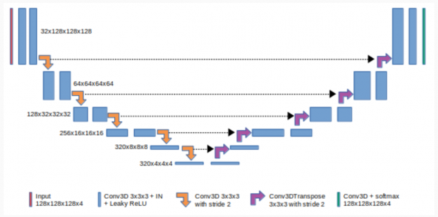
Figure 2 shows that 3D U-Net consists of a contractive (left) and expanding (right) path. It repeatedly applies unpadded convolutions followed by max pooling for downsampling.

In deep learning, a convolutional neural network (CNN) is a subset of deep neural networks, mostly used in image recognition and image processing. CNNs use deep learning to perform both generative and descriptive tasks, often using machine vision along with recommender systems and natural language processing.

Padding in CNNs refers to the number of pixels added to an image when it is processed by the kernel of a CNN. Unpadded CNNs means that no pixels are added to the image.

Pooling is a downsampling approach in CNN. Max pooling is one of common pooling methods that summarize the most activated presence of a feature. Every step in the expanding path consists of a feature map upsampling and a concatenation with the correspondingly cropped feature map from the contractive path.

Requirements

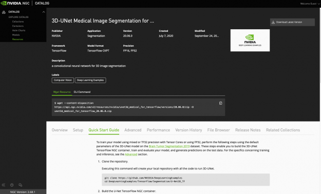
This resource contains a Dockerfile that extends the TensorFlow NGC container and encapsulates some dependencies. The resource can be downloaded using the following commands:

wget --content-disposition https://api.ngc.nvidia.com/v2/resources/nvidia/unet3d_medical_for_tensorflow/versions/20.06.0/zip -O unet3d_medical_for_tensorflow_20.06.0.zip

Aside from these dependencies, you also need the following components:

• NVIDIA Docker
• Latest TensorFlow container from NGC
• NVIDIA Ampere Architecture, NVIDIA Turing, or NVIDIA Volta GPUs

To train your model using mixed or TF32 precision with Tensor Cores or using FP32, perform the following steps using the default parameters of the 3D U-Net model on the Brain Tumor Segmentation 2019 dataset.

Download the resource

Download the resource manually by clicking the three dots at the top-right corner of the resource page.

You could also use the following wget command:

wget --content-disposition https://api.ngc.nvidia.com/v2/resources/nvidia/unet3d_medical_for_tensorflow/versions/20.06.0/zip -O unet3d_medical_for_tensorflow_20.06.0.zip

Build the U-Net TensorFlow NGC container

This command uses the Dockerfile to create a Docker image named unet3d_tf, downloading all the required components automatically.

docker build -t unet3d_tf .

Download the dataset

Data can be obtained by registering on the Brain Tumor Segmentation 2019 dataset website. The data should be downloaded and placed where /data in the container is mounted.

Run the container

To start an interactive session in the NGC container to run preprocessing, training, and inference, you must run the following command. This launches the container and mounts the ./data directory as a volume to the /data directory inside the container, mounts the ./results directory to the /results directory in the container.

The advantage of using a container is that it packages all the necessary libraries and dependencies into a single, isolated environment. This way you don’t have to worry about the complex install process.

mkdir data
mkdir results
  
docker run --runtime=nvidia -it --shm-size=1g --ulimit memlock=-1 --ulimit stack=67108864 --rm --ipc=host -v ${PWD}/data:/data -v ${PWD}/results:/results  -p 8888:8888 unet3d_tf:latest /bin/bash 

Start the notebook inside the container

Use this command to start a Jupyter notebook inside the container:

jupyter notebook --ip 0.0.0.0 --port 8888 --allow-root

Move the dataset to the /data directory inside the container. Download the notebook with the following command:

 wget --content-disposition https://api.ngc.nvidia.com/v2/resources/nvidia/med_3dunet/versions/1/zip -O med_3dunet_1.zip

Then, upload the downloaded notebook into JupyterLab and run the cells of the notebook to preprocess the dataset and train, benchmark, and test the model.

Jupyter notebook

By running the cells of this Jupyter notebook, you can first check the downloaded dataset and see the brain tumor images. After that, see the data preprocessing command and prepare the data for training. The next step is training the model and using the checkpoints of the training process for the predicting step. Finally, check the output of the predict function visually.

Checking the images

To check the dataset, you can use nibabel, which is a package that provides read/write access to some common medical and neuroimaging file formats.

By running the next three cells, you can install nibabel using pip install, choose an image from the dataset, and plot the chosen third image from the dataset using matplotlib. You can check other dataset images by changing the image address in the code.

import nibabel as nib
import matplotlib.pyplot as plt
  
img_arr = nib.load('/data/MICCAI_BraTS_2019_Data_Training/HGG/BraTS19_2013_10_1/BraTS19_2013_10_1_flair.nii.gz').get_data()
  
def show_plane(ax, plane, cmap="gray", title=None):
     ax.imshow(plane, cmap=cmap)
     ax.axis("off")
  
     if title:
         ax.set_title(title)
         
(n_plane, n_row, n_col) = img_arr.shape
_, (a, b, c) = plt.subplots(ncols=3, figsize=(15, 5))
  
show_plane(a, img_arr[n_plane // 2], title=f'Plane = {n_plane // 2}')
show_plane(b, img_arr[:, n_row // 2, :], title=f'Row = {n_row // 2}')
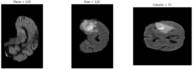
show_plane(c, img_arr[:, :, n_col // 2], title=f'Column = {n_col // 2}') 

The result is something like Figure 4.

Data preprocessing

The dataset/preprocess_data.py script converts the raw data into the TFRecord format used for training and evaluation. This dataset, from the 2019 BraTS challenge, contains over 3 TB multiinstitutional, routine, clinically acquired, preoperative, multimodal, MRI scans of glioblastoma (GBM/HGG) and lower-grade glioma (LGG), with the pathologically confirmed diagnosis. When available, overall survival (OS) data for the patient is also included. This data is structured in training, validation, and testing datasets.

The format of images is nii.gz. NIfTI is a type of file format for neuroimaging. You can preprocess the downloaded dataset by running the following command:

python dataset/preprocess_data.py -i /data/MICCAI_BraTS_2019_Data_Training -o /data/preprocessed -v

The final format of the processed images is tfrecord. To help you read data efficiently, serialize your data and store it in a set of files (~100 to 200 MB each) that can each be read linearly. This is especially true if the data is being streamed over a network. It can also be useful for caching any data preprocessing. The TFRecord format is a simple format for storing a sequence of binary records, which speeds up the data loading process considerably.

Training using default parameters

After the Docker container is launched, you can start the training of a single fold (fold 0) with the default hyperparameters (for example, {1 to 8} GPUs {TF-AMP/FP32/TF32}):

Bash examples/unet3d_train_single{_TF-AMP}.sh <number/of/gpus> <path/to/dataset> <path/to/checkpoint> <batch/size>

For example, to run with 32-bit precision (FP32 or TF32) with batch size 2 on one GPU, run the following command:

bash examples/unet3d_train_single.sh 1 /data/preprocessed /results 2

To train a single fold with mixed precision (TF-AMP) with on eight GPUs and batch size 2 per GPU, run the following command:

bash examples/unet3d_train_single_TF-AMP.sh 8 /data/preprocessed /results 2

Training performance benchmarking

The training performance can be evaluated by running benchmarking scripts:

bash examples/unet3d_{train,infer}_benchmark{_TF-AMP}.sh <number/of/gpus/for/training> <path/to/dataset> <path/to/checkpoint> <batch/size>

This script makes the model run and reports the performance. For example, to benchmark training with TF-AMP with batch size 2 on four GPUs, run the following command:

bash examples/unet3d_train_benchmark_TF-AMP.sh 4 /data/preprocessed /results 2

Predict

You can use the test dataset and predict as exec-mode to test the model. The result is saved in the model_dir directory and data_dir is the path to the dataset:

python main.py --model_dir /results --exec_mode predict --data_dir /data/preprocessed_test

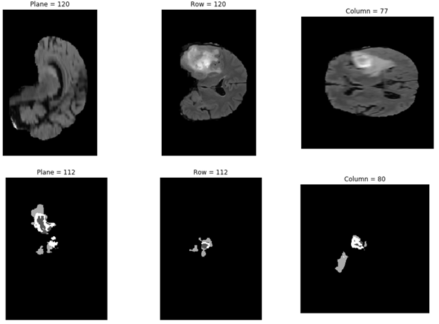
Plotting the result of prediction

In the following code example, you plot one of the chosen results from the \results folder:

import numpy as np
from mpl_toolkits import mplot3d
import matplotlib.pyplot as plt
data= np.load('/results/vol_0.npy')
def show_plane(ax, plane, cmap="gray", title=None):
     ax.imshow(plane, cmap=cmap)
     ax.axis("off")
     if title:
         ax.set_title(title)        
(n_plane, n_row, n_col) = data.shape
_, (a, b, c) = plt.subplots(ncols=3, figsize=(15, 5))
show_plane(a, data[n_plane // 2], title=f'Plane = {n_plane // 2}')
show_plane(b, data[:, n_row // 2, :], title=f'Row = {n_row // 2}')
show_plane(c, data[:, :, n_col // 2], title=f'Column = {n_col // 2}') 

Advanced options

For those of you looking to explore advanced features built into this notebook, you can see the full list of available options for main.py using -h or --help. By running the next cell, you can see how to change execute mode and other parameters of this script. You can perform model training, predicting, evaluating, and inferencing using customized hyperparameters using this script.

python main.py --help

The main.py parameters can be changed to perform different tasks, including training, evaluation, and prediction.

You can also train the model using default hyperparameters. By running the python main.py --help command, you can see the list of arguments that you can change, including training hyperparameters. For example, in training mode, you can change the learning rate from the default 0.0002 to 0.001 and the training steps from 16000 to 1000 using the following command:

python main.py --model_dir /results --exec_mode train --data_dir /data/preprocessed_test --learning_rate 0.001 --max_steps 1000

You can run other execution modes available in main.py. For example, in this post, we used the prediction execution mode of python.py by running the following command:

python main.py --model_dir /results --exec_mode predict --data_dir /data/preprocessed_test

Summary and next steps

In this post, we showed how you can get started with a medical imaging model using a simple Jupyter notebook from the NGC catalog. As you make the transition from this Jupyter notebook to building your own medical imaging workflows, consider using NVIDIA Clara Train. Clara Train includes AI-Assisted Annotation APIs and an Annotation server that can be seamlessly integrated into any medical viewer, making it AI-capable. The training framework includes decentralized learning techniques, such federated learning and transfer learning for your AI workflows.

To learn how to use these resources and kickstart your AI journey, register for the upcoming webinar with live Q&A, NVIDIA NGC Jupyter Notebook Day: Medical Imaging Segmentation.