
Artificial Neural Networks (ANN) are the fundamental building blocks of AI technology. ANNs are the basis of machine learning models; they simulate the process of learning identical to human brains. Simply put, ANNs give machines the capacity to accomplish human-like performance (and beyond) for specific tasks. This article aims to provide Data Scientists with the fundamental high-level knowledge of understanding the low-level operations involved in the functions and methods invoked when training an ANN.
As Data Scientists, we aim to solve business problems by exposing patterns in data. Often, this is done using machine learning algorithms to identify patterns and predictions expressed as a model . Selecting the correct model for a particular use case, and tuning parameters appropriately requires a thorough understanding of the problem and underlying algorithm(s). An understanding of the problem domain and the algorithms are taken under consideration to ensure that we are using the models appropriately, and interpreting results correctly.
This article introduces and explains gradient descent and backpropagation algorithms. These algorithms facilitate how ANNs learn from datasets, specifically where modifications to the network’s parameter values occur due to operations involving data points and neural network predictions.
Building an intuition
Before we get into the technical details of this post, let’s look at how humans learn.
The human brain’s learning process is complicated, and research has barely scratched the surface of how humans learn. However, the little that we do know is valuable and helpful for building models. Unlike machines, humans do not need a large quantity of data to comprehend how to tackle an issue or make logical predictions; instead, we learn from our experiences and mistakes.
Humans learn through a process of synaptic plasticity. Synaptic plasticity is a term used to describe how new neural connections are formed and strengthened after gaining new information. In the same way that the connections in the brain are strengthened and formed as we experience new events, we train artificial neural networks by computing the errors of neural network predictions and strengthening or weakening internal connections between neurons based on these errors.
Gradient Descent
Gradient Descent is a standard optimization algorithm. It is frequently the first optimization algorithm introduced to train machine learning. Let’s dissect the term “Gradient Descent” to get a better understanding of how it relates to machine learning algorithms.
A gradient is a measurement that quantifies the steepness of a line or curve. Mathematically, it details the direction of the ascent or descent of a line. Descent is the action of going downwards. Therefore, the gradient descent algorithm quantifies downward motion based on the two simple definitions of these phrases.
To train a machine learning algorithm, you strive to identify the weights and biases within the network that will help you solve the problem under consideration. For example, you may have a classification problem. When looking at an image, you want to determine if the image is of a cat or a dog. To build your model, you train your algorithm with training data with correctly labeled data samples of cats and dogs images.
While the example described above is classification, the problem could be localization or detection. Nonetheless, how well a neural network performs on a problem is modeled as a function, more specifically, a cost function; a cost or what is sometimes called a loss function measures how wrong a model is. The partial derivatives of the cost function influence the ultimate model’s weights and biases selected.
Gradient Descent is the algorithm that facilitates the search of parameters values that minimize the cost function towards a local minimum or optimal accuracy.
Cost functions, Gradient Descent and Backpropagation in Neural Networks
Neural networks are impressive. Equally impressive is the capacity for a computational program to distinguish between images and objects within images without being explicitly informed of what features to detect.
It is helpful to think of a neural network as a function that accepts inputs (data ), to produce an output prediction. The variables of this function are the parameters or weights of the neuron.
Therefore the key assignment to solving a task presented to a neural network will be to adjust the values of the weights and biases in a manner that approximates or best represents the dataset.
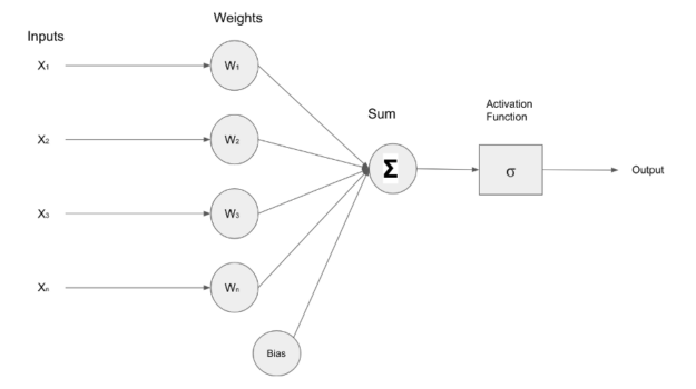
The image below depicts a simple neural network that receives input(X1, X2, X3, Xn), these inputs are fed forward to neurons within the layer containing weights(W1, W2, W3, Wn). The inputs and weights undergo a multiplication operation and the result is summed together by an adder(), and an activation function regulates the final output of the layer.
To assess the performance of neural networks, a mechanism for quantifying the difference or gap between the neural network prediction and the actual data sample value is required, yielding the calculation of a factor that influences the modification of weights and biases within a neural network.
The error gap between the predicted value of a neural network and the actual value of a data sample is facilitated by the cost function.
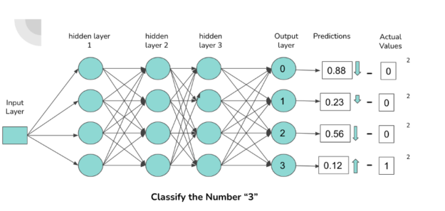
The image above illustrates a simple neural network architecture of densely connected neurons that classifies images containing the digits 0-3. Each neuron in the output layer corresponds to a digit. The higher the activations of the connection to a neuron, the higher the probability outputted by the neuron. The probability corresponds to the likelihood that the digit fed forward through the network is associated with the activated neuron.
When a ‘3’ is fed forward through the network, we expect the connections (represented by the arrows in the diagram) responsible for classifying a ‘3’ to have higher activation, which results in a higher probability for the output neuron associated with the digit ‘3’.
Several components are responsible for the activation of a neuron, namely biases, weights, and the previous layer activations. These specified components have to be iteratively modified for the neural network to perform optimally on a particular dataset.
By leveraging a cost function such as ‘mean squared error’, we obtain information in relation to the error of the network that is used to propagate updates backwards through the network’s weights and biases.
For completeness, below are examples of cost functions used within machine learning:
- Mean Squared Error
- Categorical Cross-Entropy
- Binary Cross-Entropy
- Logarithmic Loss
We have covered how to improve neural networks’ performance through a technique that measures the network’s predictions. The rest of the content in this article focuses on the relationship between gradient descent, backpropagation, and cost function.
The image in figure 3 illustrates a cost function plotted on the x and y-axis that hold values within the function’s parameter space. Let’s take a look at how neural networks learn by visualizing the cost function as an uneven surface plotted on a graph within the parameter spaces of the possible weight/parameters values.
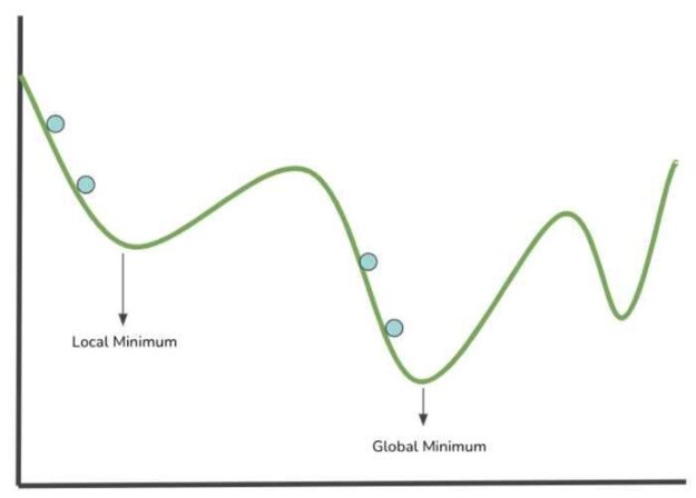
The blue points in the image above represent a step (evaluation of parameters values into the cost function) in the search for a local minimum. The lowest point of a modeled cost function corresponds to the position of weights values that results in the lowest value of the cost function. The smaller the cost function is, the better the neural network performs. Therefore, it is possible to modify the networks’ weights from the information gathered.
Gradient descent is the algorithm employed to guide the pairs of values chosen at each step towards a minimum.
- Local Minimum: The minimum parameter values within a specified range or sector of the cost function.
- Global Minimum: This is the smallest parameter value within the entire cost function domain.
The gradient descent algorithm guides the search for values that minimize the function at a local/global minimum by calculating the gradient of a differentiable function and moving in the opposite direction of the gradient.
Backpropagation is the mechanism by which components that influence the output of a neuron (bias, weights, activations) are iteratively adjusted to reduce the cost function. In the architecture of a neural network, the neuron’s input, including all the preceding connections to the neurons in the previous layer, determines its output.
The critical mathematical process involved in backpropagation is the calculation of derivatives. The backpropagation’s operations calculate the partial derivative of the cost function with respect to the weights, biases, and previous layer activations to identify which values affect the gradient of the cost function.
The minimization of the cost function by calculating the gradient leads to a local minimum. In each iteration or training step, the weights in the network are updated by the calculated gradient, alongside the learning rate, which controls the factor of modification made to weight values. This process is repeated for each step to be taken during the training phase of a neural network. Ideally, the goal is to be closer to a local minimum after each step.
The name “Backpropagation” comes from the process’s literal meaning, which is “backwards propagation of errors”. The partial derivative of the gradient quantifies the error. By propagating the errors backwards through the network, the partial derivative of the gradient of the last layer (closest layer to the output layer) is used to calculate the gradient of the second to the last layer.
The propagation of errors through the layers and the utilization of the partial derivative of the gradient from a previous layer in the current layer occurs until the first layer(closest layer to the input layer) in the network is reached.
Summary
This is just a primer on the topic of gradient descent. There is a whole world of mathematics and calculus associated with the topic of gradient descent.
Packages such as TensorFlow, SciKit-Learn, PyTorch often abstract the complexities of implementing training and optimization algorithms. Nevertheless, this does not relieve Data Scientists and ML practitioners of the requirement of understanding what occurs behind the scenes of these intelligent ‘black boxes.’
Want to explore more maths associated with backpropagation? Below are some resources to aid in your exploration:
- Neural Networks: training with backpropagation
- Backpropagation
- How the backpropagation algorithm works
Dive deeper into the world of deep learning by exploring the variety of courses available at the Nvidia Deep Learning Institute.
Thanks for reading!
