As we design deep learning networks, how can we quickly prototype the complete algorithm—including pre- and postprocessing logic around deep neural networks (DNNs) —to get a sense of timing and performance on standalone GPUs? This question comes up frequently from the scientists and engineers I work with. Traditionally, they would hand translate the complete algorithm into CUDA and compile it with the NVIDIA toolchain. However, they want to know if there’s a more automated way of short-circuiting the standard process.
Depending on the tools you’re using, compilers exist which can help automate the process of converting designs to CUDA. Engineers and scientists using MATLAB have access to tools to label ground truth and accelerate the design and training of deep learning networks that were covered in a previous post. MATLAB can also import and export using the ONNX format to interface with other frameworks. Finally, to quickly prototype designs on GPUs, MATLAB users can compile the complete algorithm to run on any modern NVIDIA GPUs, from NVIDIA Tesla to DRIVE to Jetson AGX Xavier platforms.
In this post, you’ll learn how you can use MATLAB’s new capabilities to compile MATLAB applications, including deep learning networks and any pre- or postprocessing logic, into CUDA and run it on modern NVIDIA GPUs.
Let’s use a traffic sign detection recognition (TSDR) example to show the steps in the workflow:
- Run and test algorithm in MATLAB
- Compile algorithm to CUDA and run on desktop GPU
- Compile algorithm to CUDA and integrate with external applications
Traffic Sign Detection and Recognition Algorithm
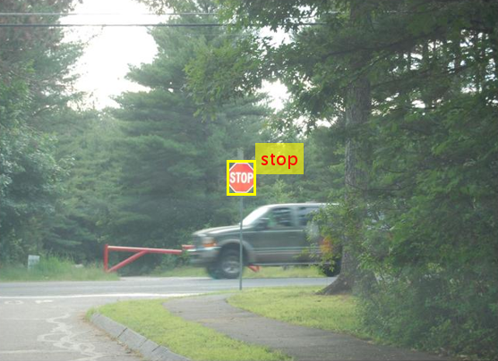
The goal of the algorithm is to detect and recognize traffic signs using cameras mounted on vehicles. We feed in input images or video to the algorithm and it returns with a listing of traffic signs detected in the input. Traffic signs are also identified by a box in the output image. Figure 1 shows a test image and successful detection of a stop sign.
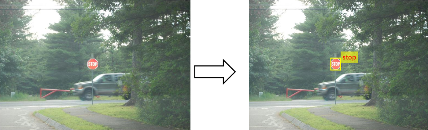
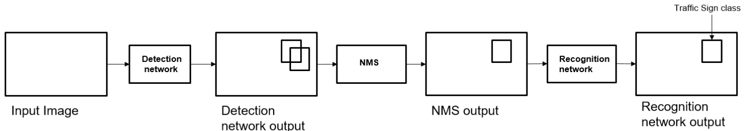
Figure 2 shows the traffic sign detection and recognition happens in three steps: detection, Non-Maximal Suppression (NMS), and recognition. First, the detection network (a variant of the You Only Look Once (YOLO) network) detects traffic signs from input images. Overlapping detections from the preceding stage are then suppressed using the NMS algorithm. Finally, the recognition network classifies the detected traffic signs.
Detection and Recognition Networks
The detection network is trained in the Darknet framework and imported into MATLAB for inference. All traffic signs are considered as a single class for training the detection network since the size of the traffic sign is small relative to that of the image and the number of training samples per class are less in the training data.
The detection network divides the input image into a 7 x 7 grid and each grid cell detects a traffic sign if the center of the traffic sign falls within the grid cell. Each cell predicts two bounding boxes and confidence scores for these bounding boxes. Confidence scores tell us whether the box contains an object or not. Each cell also predicts the probability for finding the traffic sign in the grid cell. The final score is product of the above two. We apply a threshold of 0.2 on this final score to select the detections.
The detection network contains 58 layers, including convolution, leaky ReLU, and fully connected layers. Table 1 shows a snippet of the layers displayed in MATLAB.
| 58×1 Layer array with layers: | |||
| 1 | ‘input’ | Image Input | 448x448x3 images |
| 2 | ‘conv1’ | Convolution | 64 7x7x3 convolutions with stride [2 2] and padding [3 3 3 3] |
| 3 | ‘relu1’ | Leaky ReLU | Leaky ReLU with scale 0.1 |
| 4 | ‘pool1’ | Max Pooling | 2×2 max pooling with stride [2 2] and padding [0 0 0 0] |
| 5 | ‘conv2’ | Convolution | 192 3x3x64 convolutions with stride [1 1] and padding [1 1 1 1] |
| 6 | ‘relu2’ | Leaky ReLU | Leaky ReLU with scale 0.1 |
| 7 | ‘pool2’ | Max Pooling | 2×2 max pooling with stride [2 2] and padding [0 0 0 0] |
| 8 | ‘conv3’ | Convolution | 128 1x1x192 convolutions with stride [1 1] and padding [0 0 0 0] |
| 9 | ‘relu3’ | Leaky ReLU | Leaky ReLU with scale 0.1 |
| 10 | ‘conv4’ | Convolution | 256 3x3x128 convolutions with stride [1 1] and padding [1 1 1 1] |
| 11 | ‘relu4’ | Leaky ReLU | Leaky ReLU with scale 0.1 |
| 12 | ‘conv5’ | Convolution | 256 1x1x256 convolutions with stride [1 1] and padding [0 0 0 0] |
| 13 | ‘relu5’ | Leaky ReLU | Leaky ReLU with scale 0.1 |
| 14 | ‘conv6’ | Convolution | 512 3x3x256 convolutions with stride [1 1] and padding [1 1 1 1] |
| 15 | ‘relu6’ | Leaky ReLU | Leaky ReLU with scale 0.1 |
| 16 | ‘pool6’ | Max Pooling | 2×2 max pooling with stride [2 2] and padding [0 0 0 0] |
Table 1. A snippet of the 58 layers in the detection network
The recognition network is trained on the same images using MATLAB and contains 14 layers, including convolution, fully connected, and classification output layers. Table 2 shows details of the layers displayed in MATLAB.
| 14×1 Layer array with layers: | |||
| 1 | ‘imageinput’ | Image Input | 48x48x3 images with ‘zerocenter’ normalization and ‘randfliplr’ augmentations |
| 2 | ‘conv_1’ | Convolution | 100 7x7x3 convolutions with stride [1 1] and padding [0 0 0 0] |
| 3 | ‘relu_1’ | ReLU | ReLU |
| 4 | ‘maxpool_1’ | Max Pooling | 2×2 max pooling with stride [2 2] and padding [0 0 0 0] |
| 5 | ‘conv_2’ | Convolution | 150 4x4x100 convolutions with stride [1 1] and padding [0 0 0 0] |
| 6 | ‘relu_2’ | ReLU | ReLU |
| 7 | ‘maxpool_2’ | Max Pooling | 2×2 max pooling with stride [2 2] and padding [0 0 0 0] |
| 8 | ‘conv_3’ | Convolution | 250 4x4x150 convolutions with stride [1 1] and padding [0 0 0 0] |
| 9 | ‘maxpool_3’ | Max Pooling | 2×2 max pooling with stride [2 2] and padding [0 0 0 0] |
| 10 | ‘fc_1’ | Fully Connected | 300 fully connected layer |
| 11 | ‘dropout’ | Dropout | 90% dropout |
| 12 | ‘fc_2’ | Fully Connected | 35 fully connected layer |
| 13 | ‘softmax’ | Softmax | Softmax |
| 14 | ‘classoutput’ | Classification Output | crossentropyex with ‘0’ and 34 other classes |
Table 2. The 14 layers of the recognition network
Run and Test Algorithm in MATLAB
The TSDR algorithm is defined in the tsdr_predict.m function. The function starts by converting the input image into BGR format before sending it to the detection network, which is specified in yolo_tsr.mat. The function loads network objects from yolo_tsr.mat into a persistent variable detectionnet so persistent objects are reused on subsequent calls to the function.
function [selectedBbox,idx] = tsdr_predict(img)
coder.gpu.kernelfun;
img_rz = imresize(img,[448,448]);   % Resize the image
img_rz = img_rz(:,:,3:-1:1);        % Converting into BGR format
img_rz = im2single(img_rz);

%% Traffic sign detection
persistent detectionnet;
if isempty(detectionnet)
   detectionnet = coder.loadDeepLearningNetwork('yolo_tsr.mat','Detection');
end
predictions = detectionnet.activations(img_rz,56,'OutputAs','channels');
The function then takes the output from the detection network to find bounding box coordinates in the input image before suppressing overlapping detections using selectStrongestBbox function.
coder.varsize('selectedBbox',[98, 4],[1 0]);
[selectedBbox,~] = selectStrongestBbox(round(boxes),probs);
Finally, the function recognizes traffic signs using the recognition network. As before with detectionnet, the function loads the network objects from recognitionNet.mat into a persistent variable recognitionnet so persistent objects are reused on subsequent calls.
persistent recognitionnet;
if isempty(recognitionnet)
   recognitionnet = coder.loadDeepLearningNetwork('RecognitionNet.mat','Recognition');
end

idx = zeros(size(selectedBbox,1),1);
inpImg = coder.nullcopy(zeros(48,48,3,size(selectedBbox,1)));
for i = 1:size(selectedBbox,1)

   ymin = selectedBbox(i,2);
   ymax = ymin+selectedBbox(i,4);
   xmin = selectedBbox(i,1);
   xmax = xmin+selectedBbox(i,3);

   % Resize Image
   inpImg(:,:,:,i) = imresize(img(ymin:ymax,xmin:xmax,:),[48,48]);

end

for i = 1:size(selectedBbox,1)
   output = recognitionnet.predict(inpImg(:,:,:,i));
   [~,idx(i)]=max(output);
end
To test tsdr_predict.m running in MATLAB using the CPU, we can write a test script that feeds a test image to tsdr_predict, then map class numbers to the class dictionary to get the type of traffic sign detected. We then draw a bounding box around the detected traffic sign and label it on the output image. The result from running the test script below is the same output image shown in Figure 1.
im = imread('stop.jpg');
im = imresize(im, [480,704]);
[bboxes,classes] = tsdr_predict_mex(im);

% Map the class numbers to traffic sign names in the class dictionary.
classNames = {'addedLane','slow','dip','speedLimit25','speedLimit35','speedLimit40','speedLimit45',...
   'speedLimit50','speedLimit55','speedLimit65','speedLimitUrdbl','doNotPass','intersection',...
   'keepRight','laneEnds','merge','noLeftTurn','noRightTurn','stop','pedestrianCrossing',...
   'stopAhead','rampSpeedAdvisory20','rampSpeedAdvisory45','truckSpeedLimit55',...
   'rampSpeedAdvisory50','turnLeft','rampSpeedAdvisoryUrdbl','turnRight','rightLaneMustTurn',...
   'yield','yieldAhead','school','schoolSpeedLimit25','zoneAhead45','signalAhead'};

classRec = classNames(classes);
outputImage = insertShape(im,'Rectangle',bboxes,'LineWidth',3);

for i = 1:size(bboxes,1)
   outputImage = insertText(outputImage,[bboxes(i,1)+bboxes(i,3) bboxes(i,2)-20],classRec{i},...
      'FontSize',20,'TextColor','red');
end
figure;
imshow(outputImage);
Compile Algorithm to CUDA and Run on Desktop GPU
Having tested the algorithm successfully in MATLAB on the CPU, the next step is to improve performance by running the algorithm on GPUs. Let’s begin by using the newly released MATLAB GPU Coder to compile the complete algorithm into CUDA. We first create a GPU configuration object for MEX files, which is source code compiled for use in MATLAB. We can specify the configuration to use either cuDNN or TensorRT with INT8 datatypes:
cfg.DeepLearningConfig = coder.DeepLearningConfig('cudnn');     % Use cuDNN
cfg.DeepLearningConfig = coder.DeepLearningConfig('tensorrt');  % Use TensorRT
Let’s use TensorRT. We’ll run the codegen command to start the compilation and specify the input to be of size [480,704,3] and type uint8. This value corresponds to the input image size of tsdr_predict function. GPU Coder then creates a MEX file, tsdr_predict_mex.
cfg = coder.gpuConfig('mex');
cfg.TargetLang = 'C++';
cfg.DeepLearningConfig = coder.DeepLearningConfig('tensorrt');
codegen -config cfg tsdr_predict -args {ones(480,704,3,'uint8')} -report
To test the MEX file, we reuse the same test script shown in the preceding section. We make one change to use tsdr_predict_mex instead of tsdr_predict.
[bboxes,classes] = tsdr_predict_mex(im);
The result from running tsdr_predict_mex is the same as running tsdr_predict. The output image matches the one shown in Figure 1 with a bounding box around the labeled traffic sign.
We can further test the algorithm on suites of test images and videos; MATLAB provides various facilities for accessing data stored locally, on networks, and in the cloud. We can even bring in live images and video using cameras connected to our testing machines. MATLAB also provides a unit test framework to help set up and run tests in a systematic way.
Compare Performance Gain of TensorRT and cuDNN
Earlier, we mentioned we can compile tsdr_predict.m to use cuDNN or TensorRT. Let’s take a look at the performance gain of using TensorRT relative to that of using cuDNN. We will use the same machine fitted with a Titan V GPU and Intel Xeon processor to time the results.
First, let’s record the execution time of the current MEX file using TensorRT with the help of the MATLAB timeit function. Averaged over 10 executions, we see an execution time of 0.0107s, which is equivalent to about 93 images/sec.
f = @() tsdr_predict_mex(im);
measured_time=0;
for i = 1:10
    measured_time = measured_time + timeit(f);
end
measured_time = measured_time/10;
Next, let’s time the execution time of the MEX file that uses cuDNN. We will retrace our steps and configure GPU Coder to use cuDNN to create the MEX file.
cfg = coder.gpuConfig('mex');
cfg.TargetLang = 'C++';
cfg.DeepLearningConfig = coder.DeepLearningConfig('cudnn');
codegen -config cfg tsdr_predict -args {ones(480,704,3,'uint8')} -report
We then use the same timeit function to run the MEX file using cuDNN. When averaged over 10 executions, we see an execution time of 0.0131s, which is approximately 76 images/sec. Comparing these two results, we see that using TensorRT with INT8 resulted in an increase of 93/76 = 22% for single image inference using two moderately sized networks. Table 3 summarizes the execution time of running on the CPU and GPU (Titan V) with cuDNN and TensorRT.
| CPU | GPU with cuDNN | GPU with TensorRT (INT8) | |
| Execution time (s) | 0.0320s | 0.0131s | 0.0107s |
| Equivalent images/sec | 31 | 76 | 93 |
Table 3. Timing results of running tsdr_predict on CPU (Intel® Xeon CPU @ 3.6 GHz) and GPU (Titan V) with cuDNN and TensorRT
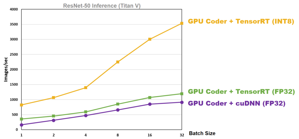
As an aside, we benchmarked results of using GPU Coder with cuDNN and TensorRT on ResNet-50 using the same Titan V GPU. The results are shown in Figure 3. We found that TensorRT INT8 datatype mode increases inference performance, especially at higher batch sizes:
Compile Algorithm to CUDA and Integrate with External Applications
Once we made sure the algorithm ran correctly in MATLAB on our desktop GPU, we could compile the algorithm to source code or a library to integrate into larger applications. Let’s configure GPU Coder to compile the algorithm into a library.
cfg = coder.gpuConfig('lib');
cfg.TargetLang = 'C++';
cfg.DeepLearningConfig = coder.DeepLearningConfig('tensorrt');
codegen -config cfg tsdr_predict -args {ones(480,704,3,'uint8')} -report
GPU Coder then creates a static library, tsdr_predict.a. You can integrate this library with applications running on your host machine, in the cloud, or even run it on mobile and embedded systems like the Jetson Xavier.
GPU Coder provides an example main function to show how you can call the library from your application. You need to call the initialization once before calling the tsdr_predict function. Finally, you should call the terminate function to free up resources for other applications when done.
int32_T main(int32_T, const char * const [])
{
   // Initialize the application.
   // You do not need to do this more than one time.
   tsdr_predict_initialize();

   // Invoke the entry-point functions.
   // You can call entry-point functions multiple times.
   main_tsdr_predict();

   // Terminate the application.
   // You do not need to do this more than one time.
   tsdr_predict_terminate();
   return 0;
}
static void main_tsdr_predict()
{
   real32_T selectedBbox_data[392];
   int32_T selectedBbox_size[2];
   real_T idx_data[98];
   int32_T idx_size[1];
   static uint8_T b[1013760];

   // Initialize function 'tsdr_predict' input arguments.
   // Initialize function input argument 'img'.
   // Call the entry-point 'tsdr_predict'.
   argInit_480x704x3_uint8_T(b);
   tsdr_predict(b, selectedBbox_data, selectedBbox_size, idx_data, idx_size);
}
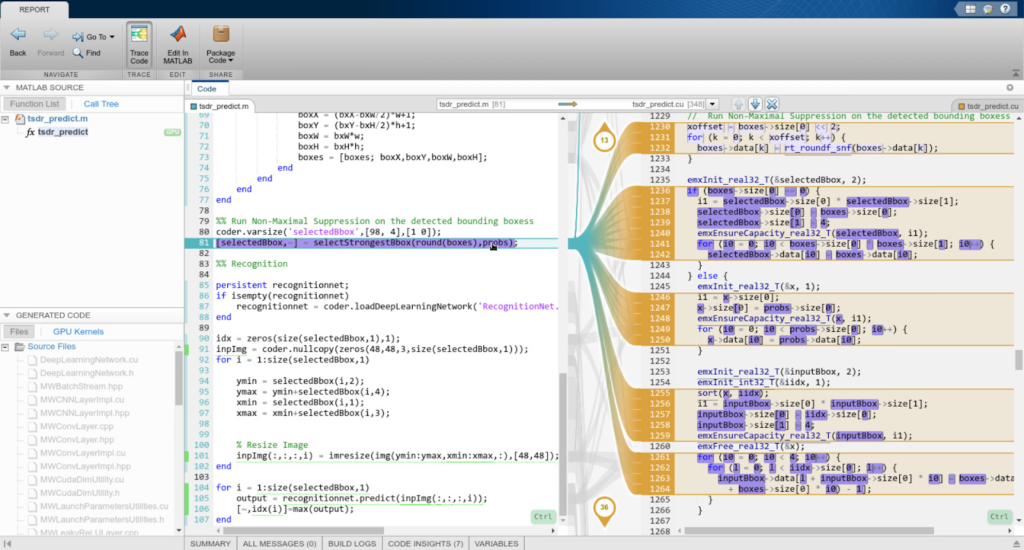
Examine the Source Code
For those inclined, we can take a deeper look at the source code, which is stored in the same folder as the library. GPU Coder creates a code generation report that provides an interface to examine the original MATLAB code and generated CUDA code. The report also provides a handy interactive code traceability tool to map between MATLAB code and CUDA. Figure 4 shows a screen capture of the tool in action.
Let’s examine parts of the compiled CUDA code. Starting with the header file tsdr_predict.h, we see there are two function declarations.
// Include Files
#include <stddef.h>
#include <stdlib.h>
#include "rtwtypes.h"
#include "tsdr_predict_types.h"

// Function Declarations
extern void tsdr_predict(const uint8_T img[1013760], real32_T selectedBbox_data[],
   int32_T selectedBbox_size[2], real_T idx_data[], int32_T idx_size[1]);
extern void tsdr_predict_init();
...
Looking inside the source file tsdr_predix.cu, we can find the tsdr_predict function. The code snippet below shows the beginning of the function.
void tsdr_predict(const uint8_T img[1013760], real32_T selectedBbox_data[],
                  int32_T selectedBbox_size[2], real_T idx_data[], int32_T
                  idx_size[1])
{
   int32_T auxLength;
   int32_T rowIdx;
   int32_T colIdx;
   int32_T l;
   real_T sumVal;
   real_T absx2;
   int32_T numOfBbox;
   real_T oldIdx;
   int32_T xoffset;

...
Memory allocation is taken care of through cudaMalloc calls, which the following code snippet shows.
boolean_T exitg1;
cudaMalloc(&gpu_inpImg, 55296UL);
cudaMalloc(&gpu_inpImg_data, 677376U * sizeof(uint8_T));
cudaMalloc(&b_gpu_partialResize_size, 12UL);
cudaMalloc(&d_gpu_ResizedImage, 6912UL);
cudaMalloc(&gpu_partialResize_size, 12UL);
cudaMalloc(&b_gpu_colWeightsTotal, 384UL);
cudaMalloc(&b_gpu_rowWeightsTotal, 384UL);
...
Looking further down, GPU Coder generated several kernels for resizing the image. Data is moved between CPU and GPU memory spaces through cudaMemcpy calls at the appropriate locations to minimize data copies. Code snippets for part of the operation is shown below.
cudaMemcpy(gpu_img, (void *)&img[0], 1013760UL, cudaMemcpyHostToDevice);
tsdr_predict_kernel9<<<dim3(1260U, 1U, 1U), dim3(512U, 1U, 1U)>>>
   (*gpu_colWeightsTotal, *gpu_colWeights, *gpu_img, *gpu_ipColIndices,*gpu_partialResize);
tsdr_predict_kernel10<<<dim3(1176U, 1U, 1U), dim3(512U, 1U, 1U)>>>
   (*gpu_rowWeightsTotal, *gpu_rowWeights, *gpu_partialResize, *gpu_ipRowIndices, *gpu_ResizedImage);
...
Using the code traceability tool, we find the recognition network is defined in the DeepLearningNetwork_predict function. Inside, cudaMalloc calls are used to move data to GPU memory before launching several CUDA kernels. Data is moved back to CPU memory following the CUDA kernels using cudaMalloc, followed by cudaFree calls to free up GPU memory.
void DeepLearningNetwork_predict(b_Recognition_0 *obj, const real_T inputdata [6912], real32_T outT[35])
{
   real32_T (*gpu_inputT)[6912];
   real32_T (*gpu_out)[35];
   real_T (*gpu_inputdata)[6912];
   real32_T (*b_gpu_inputdata)[6912];
   real32_T (*gpu_outT)[35];
   cudaMalloc(&gpu_outT, 140UL);
   cudaMalloc(&gpu_out, 140UL);
   cudaMalloc(&gpu_inputT, 27648UL);
   cudaMalloc(&b_gpu_inputdata, 27648UL);
   cudaMalloc(&gpu_inputdata, 55296UL);
   cudaMemcpy(gpu_inputdata, (void *)&inputdata[0], 55296UL, cudaMemcpyHostToDevice);
c_DeepLearningNetwork_predict_k<<<dim3(14U, 1U, 1U), dim3(512U, 1U, 1U)>>>
   (*gpu_inputdata, *b_gpu_inputdata);
d_DeepLearningNetwork_predict_k<<<dim3(14U, 1U, 1U), dim3(512U, 1U, 1U)>>>
   (*b_gpu_inputdata, *gpu_inputT);
cudaMemcpy(obj->inputData, *gpu_inputT, 6912UL * sizeof(real32_T),cudaMemcpyDeviceToDevice);
obj->predict();
cudaMemcpy(*gpu_out, obj->outputData, 35UL * sizeof(real32_T), cudaMemcpyDeviceToDevice);
e_DeepLearningNetwork_predict_k<<<dim3(1U, 1U, 1U), dim3(64U, 1U, 1U)>>>
   (*gpu_out, *gpu_outT);
...
GPU Coder also generates CUDA kernels for other parts of the TSDR function to accelerate the algorithm. In total, GPU Coder created 31 CUDA kernels. The code generation report provides a listing of the kernels, along with other pertinent information.
Conclusion
In this post, we’ve covered how to run and test algorithms in MATLAB before compiling them to CUDA and accelerating them on GPUs. The generated CUDA can also be exported from MATLAB as source code or libraries and integrated with external applications running on any modern NVIDIA GPUs, from NVIDIA Tesla to DRIVE to Jetson AGX Xavier platforms. We hope this has helped you appreciate how automated CUDA compilers like GPU Coder can help short-circuit the standard process of hand translating designs into CUDA, as well as the ease by which you can tap into the powerful performance gains provided by TensorRT.
To solve the problems described in this post, I used MATLAB R2018b along with Deep Learning Toolbox, Parallel Computing Toolbox, Computer Vision System Toolbox, GPU Coder, and, of course, the NVIDIA tools, including TensorRT. You can learn more about deep learning with MATLAB and download a free 30-day trial of MATLAB using this link.
Join Us at GTC Europe 2018
Are you attending the GTC Europe conference this year? We will present a talk and have a booth in the exhibit hall with various examples running live on NVIDIA GPUs using MATLAB and GPU Coder to develop deep learning and AI applications. We will be showing the demos from this post and more at Booth Number S06.