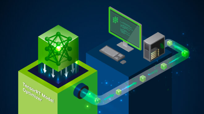
Top 5 AI Model Optimization Techniques for Faster, Smarter Inference

As AI models get larger and architectures more complex, researchers and engineers are continuously finding new techniques to optimize the performance and overall cost of bringing AI systems to production.

Model optimization is a category of techniques focused on addressing inference service efficiency. These techniques represent the best “bang for buck” opportunities to optimize cost, improve user experience, and scale. These techniques range from fast and effective approaches like model quantization to powerful multistep workflows like pruning and distillation.

This post covers the top five model optimization techniques enabled through NVIDIA Model Optimizer and how each contributes to improving the performance, TCO, and scalability of deployments on NVIDIA GPUs.

These techniques are the most powerful and scalable levers currently available in Model Optimizer that teams can apply immediately to reduce cost per token, improve throughput, and accelerate inference at scale.

A visual showing five cards, each with a small green-themed icon and headline. The techniques listed are: Post-Training Quantization (“Fastest Path to Optimization”), Quantization-Aware Training (“Simple Accuracy Recovery”), Quantization-Aware Distillation (“Max Accuracy and Speedup”), Speculative Decoding (“Speedup without Model Changes”), and Pruning & Distillation (“Slim Model and Keep Intelligence”). All cards use clean white backgrounds with NVIDIA-style green bar/brain/network iconography. — *Figure 1. The top five most impactful model optimization techniques*

1. Post-training quantization

Post-training quantization (PTQ) is the fastest path to model optimization. You can leverage an existing model (FP16/BF16/FP8) and compress it to a lower precision format (FP8, NVFP4, INT8, INT4) using a calibration dataset—without touching the original training loop. This is where most teams should begin. It is easy to apply with Model Optimizer, and delivers immediate latency plus throughput wins, even on massive foundation models.

Comparison of representable ranges and data precision for FP16, FP8, and FP4 formats. FP16 shows the widest range (−65,504 to +65,504) with closely spaced values A and B, representing high precision. FP8 has a narrower range (−448 to +448) with quantized values QA and QB spaced farther apart, indicating lower precision. FP4 shows an even smaller range (−6 to +6), illustrating the trade‑off between range and precision when reducing bit width. — *Figure 2. What happens to range and detail when quantizing from FP16 down to FP*8 or FP4

Pros	Cons
–Fastest time to value –Achievable with small calibration dataset –Memory, latency, and throughput gains stack with other optimizations –Highly custom quantization recipes (NVFP4 KV Cache, for example)	–May require a different technique (QAT/QAD) if the quality floor drops under SLA

Table 1. Pros and cons of PTQ

To learn more, see Optimizing LLMs for Performance and Accuracy with Post-Training Quantization.

2. Quantization-aware training

Quantization-aware training (QAT) injects a short, targeted fine-tuning phase where the model is tuned to account for low precision error. It simulates quantization noise in the forward loop while computing gradients in higher precision. QAT is a recommended next step when additional accuracy is required beyond what PTQ has delivered.

Flowchart illustrating the Quantization Aware Training (QAT) workflow. On the left, an original precision model is combined with calibration data and a Model Optimizer quantization recipe to form a QAT-ready model. This model, along with a subset of original training data, enters the QAT training loop. Inside the loop, high-precision weights are updated and then used as “fake quantization” weights during the forward pass. Training loss is calculated, and the backward pass uses a straight-through estimator (STE) to propagate gradients. The loop repeats until training converges. — *Figure 3.* A model is prepared, quantized, and iteratively trained with simulated low-precision weights in a QAT workflow

Pros	Cons
–Recovers all or most of the accuracy loss at low precision –Fully compatible with NVFP4, especially for FP4 stability	–Requires training budget plus data –Takes longer to implement than PTQ alone

Table 2. Pros and cons of QAT

To learn more, see How Quantization-Aware Training Enables Low-Precision Accuracy Recovery.

3. Quantization-aware distillation

Quantization-aware distillation (QAD) goes one level beyond QAT. With this technique, the student model learns to account for quantization errors while simultaneously aligned to the full precision teacher through distillation loss. QAD doubles down on QAT by adding teaching elements from principles of distillation, enabling you to extract the maximum quality possible while running ultra-low precision at inference time. QAD is an effective option for downstream tasks that notoriously suffer from significant performance degradation after quantization.

Flowchart of Quantization Aware Distillation (QAD). On the left, an original precision model is combined with calibration data and a quantization recipe to create a QAD-ready student model. This student model is paired with a higher precision teacher model and a subset of the original training data. In the QAD training loop, the student uses “fake quantization” weights in its forward pass, while the teacher performs a standard forward pass. Outputs are compared to calculate QAD loss, which combines distillation loss with standard training loss. Gradients flow back through the student model using a straight-through estimator (STE), and the student’s high-precision weights are updated to adapt to quantization conditions. — *Figure 4.* QAD trains a low-precision student model under teacher guidance, combining distillation loss with standard QAT updates

Pros	Cons
–Highest accuracy recovery –Ideal for multistage post-training pipelines for easy setup and robust convergence	–Additional training cycles after pretraining –Larger memory footprint –Slightly more complex pipeline to implement today

Table 3. Pros and cons of QAD

To learn more, see How Quantization-Aware Training Enables Low-Precision Accuracy Recovery.

4. Speculative decoding

The decode step in inference is well known for suffering from sequential processing algorithmic bottlenecks. Speculative decoding tackles this directly by using a smaller or faster draft model (like EAGLE-3) to propose multiple tokens ahead, then verifying them in parallel with the target model. This collapses sequential latency into single steps and dramatically reduces required forward passes at long sequence lengths, without touching model weights.

Speculative decoding is recommended when you want immediate generation speedups without retraining or quantization, and it stacks cleanly with the other optimizations in this list to compound throughput and latency gains.

A gif showing an example where the input is “The Quick”. From this input, the draft model proposes “Brown”, “Fox”, “Hopped”, “Over”. The input and draft are ingested by the target model, which verifies “Brown” and “Fox” before rejecting “Hopped” and subsequently everything after. “Jumped” is the target model’s own generation resulting from the forward pass. — *Figure 5. The draft-target approach to speculative decoding operates as a two-model system*

Pros	Cons
–Radically reduces decode latency –Stacks perfectly with PTQ/QAT/QAD plus NVFP4	–Requires tuning (acceptance rate is everything) –Second model or head required depending on variant

Table 4. Pros and cons of speculative decoding

To learn more, see An Introduction to Speculative Decoding for Reducing Latency in AI Inference.

5. Pruning plus knowledge distillation

Pruning is a structural optimization path. This technique removes weights, layers, and/or heads to make the model smaller. Distillation then teaches the new smaller model how to think like the larger teacher. This multistep optimization strategy permanently changes model performance because the baseline compute and memory footprint are permanently lowered.

Pruning plus knowledge distillation can be leveraged when other techniques in this list are unable to deliver the memory or compute savings necessary to meet application requirements. This approach can also be used when teams are open to making more aggressive changes to an existing model to adapt it for specific specialized downstream use cases.

This diagram shows the successful outcome of knowledge distillation by comparing the teacher network to the smaller, trained student network. The student model, despite being more compact, produces an output probability vector that closely mimics the teacher's vector. — *Figure 6. Knowledge distillation-trained student and teacher model outputs*

Pros	Cons
–Reduces parameter count → permanent plus structural cost savings –Enables smaller models that still behave like large models	–Aggressive pruning without distill → cliffs accuracy –Requires more work to pipeline versus PTQ alone

Table 5. Pros and cons of pruning plus knowledge distillation

To learn more, see Pruning and Distilling LLMs Using NVIDIA TensorRT Model Optimizer.

Get started with AI model optimization

Optimization techniques come in all shapes and sizes. This post highlights the top five model optimization techniques enabled through Model Optimizer.

PTQ, QAT, QAD, and pruning plus distillation make your model intrinsically cheaper, smaller, and more memory efficient to operate.
Speculative decoding makes generation intrinsically faster by collapsing sequential latency.

To get started and learn more, explore the deep-dive posts associated with each technique for technical explainers, performance insights, and Jupyter Notebook walkthroughs.