
RAPIDS cuML provides scalable, GPU-accelerated machine learning models with a Python interface based on the scikit-learn API. This guide will walk through how to easily train cuML models on multi-node, multi-GPU (MNMG) clusters managed by Google’s Kubernetes Engine (GKE) platform. We will examine a subset of the available MNMG algorithms, illustrate their use of leveraging Dask on a large public dataset and provide a series of code samples for exploring and recording their performance.
Dask as our distributed framework
Our first task will be to bring up our Dask cluster within Kubernetes. This will provide us with the ability to run distributed algorithms in a MNMG environment, and explore some of the implications this has on how we design our workflows, do analysis, and build models.
MNMG cuML and XGBoost
Once our Dask cluster is up and running, and we’ve had a chance to load some data and get a feel for the major ideas, we’ll take a look at the machine learning models RAPIDS has available, the flavors they come in: out-of-band and in-framework, and go through the process of training some of those models and looking at their performance in our cluster.
Pre-Requisites
Before we get started, we need to have a few pieces of software and a running Kubernetes cluster. I’ll provide a quick run through for spinning one up in GKE on Google’s Cloud Platform (GCP) as well as this more detailed guide; if you’re interested in more details about GCP or Kubernetes, I encourage you to to look into the links at the end of this guide.
Software
Local Environment
Python versioning and package manager. You’ll want to create a new environment (which the rapids install command below does).
- RAPIDS 0.19 python libraries
$ conda create -n rapids-core-0.19 -c rapidsai -c nvidia -c conda-forge \
    -c defaults cuml=0.19 python=3.8 cudatoolkit=11.0
- RAPIDS 0.19 docker container
We’ll modify this to be our scheduler/worker deployment container for our Dask cluster.
$ docker pull rapidsai/rapidsai-core:0.19-cuda11.0-runtime-ubuntu18.04-py3.8
- Dask-kubernetes, Dask_labextension, gcsfs, jupyterlab, tqdm, nodejs, xgboost, and seaborn python libraries
File system interface to GCP’s cloud storage (GCS) system.
$ conda activate rapids-core-0.19
$ conda install -c conda-forge dask-kubernetes gcsfs jupyterlab nodejs
$ pip install xgboost seaborn dask_labextension tqdm
This adds a plugin to Jupyter that lets us see what our Dask cluster is doing in real time. Very handy.
$ jupyter labextension install dask-labextension
- Add rapids-core-0.19 to JupyterLab as a selectable kernel
$ python -m ipykernel install --user --name rapids-core-0.19 --display-name "RAPIDS-0.19"
- Pull the latest notebook code and specification files from rapids cloud-ml-examples. Relevant files are found in dask/kubernetes
$ git clone https://github.com/rapidsai/cloud-ml-examples.git
At this point, you’ve got a RAPIDS-0.19 conda environment, configured with all the libraries we need, and quality of life updates for Jupyter that will make the Dask experience more interactive.
Next up: what data are we using and where do we get it?
Data
For this guide, we’ll be using a subset of the public NYC-Taxi dataset, hosted on GCS by Anaconda. The data can be accessed directly from ‘gcs://anaconda-public-data/nyc-taxi’, and can be explored easily with the gsutil utility.
$ gsutil ls -r gs://anaconda-public-data/nyc-taxi
We’ll examine a medium-sized, 150 million record set, stored in parquet format, and the larger, ~450 million record set, for 2014, 2015, 2016 saved in CSV format. This will give us a chance to observe the substantial benefit associated with selecting the proper storage format.
Kubernetes on GKE
- Create a GCP account
- Create a GKE cluster
- Allocate a node pool with at least three nodes: one for our Dask scheduler and two for workers.
- Nodes should be n1-standard-4 or greater with an attached GPU that has a compute capability of 6.0+ (we’ll use T4’s in this guide).
- Configure Kubectl and install a CUDA 11.0 compatible driver daemon.
- Authenticate Docker with your GCR account
Optional: The steps below need to be completed to allow distributed inference using the Forest Inference Library, or for experimenting with the parquet converted mortgage data.
Configuring our Dask Cluster
Before we can launch our Dask cluster we need to create our scheduler/worker container and push it to GCR and update our Dask-Kubernetes configuration files to reflect your specific Kubernetes cluster.
Cluster specific items
- Navigate to the cloud-ml-examples repo you downloaded in the ‘Local Environment’ step above.
$ cd Dask/kubernetes
$ ls
Dask_Cuml_Exploration.ipynb Dockerfile specs- Build your scheduler/worker container, tag it with the gcr path corresponding to your GCP project, and push your GCR repo.
$ docker build --tag gcr.io/${YOUR_PROJECT}/${YOUR_REPO}/dask-unified:0.19 --file Dockerfile .
$ docker push gcr.io/${YOUR_PROJECT}/${YOUR_REPO}/dask-unified:0.19- Update the two yaml files sched-spec.yaml and worker-spec.yaml found in ./spec
- Find the image entry under the containers block and set it to your GCR image path. Next, locate the limits and requests blocks and set their cpu and memory elements based on available resources in your cluster.
For example, n1-standard-4 has 4 vcpus, and 15 GB of memory, so we might configure our container specification as follows (you can find the exact amount of allocatable resources in the GCP console by looking at the ‘Nodes’ table in your cluster details).
containers:
   - image: gcr.io/${YOUR_PROJECT}/${YOUR_REPO}/Dask-unified:0.19
   … SNIP …
   resources:
     limits:
       cpu: “3”
       memory: 13G
       nvidia.com/gpu: 1
     requests:
       cpu: “3”
       memory: 13G
Deploy the cluster
At this point, we’re finished with all the configuration elements and can start exploring the code. I’ll reference the relevant bits here, and you can refer to the underlying notebook for additional details. To get started, bring up a jupyter lab notebook instance on your workstation and open ‘Dask_cuML_Exploration.ipynb’.
- Make sure you select the RAPIDS-0.19 kernel we installed previously.
![]()
![]()
- Run the first three cells to launch your Dask cluster. These will:
- Create scheduler and worker pod templates from ‘sched-spec.yaml’ and ‘worker-spec.yaml’.
- Create a cluster from the pod templates, attach a Dask client, and scale up the cluster to have two workers.
cluster = KubeCluster(pod_template=worker_pod,
                      scheduler_pod_template=sched_pod)

client = Client(cluster)

n_workers = 2
cluster.scale(n_workers)
Note: This process may take 5-10 minutes for the first run, as each worker will need to pull its container.
- During this time, it can be useful to open a separate terminal window and monitor your kubernetes activity with kubectl. This will also allow you to get the external-ip of the Dask scheduler, once it’s created and being monitoring the cluster.
$ watch kubectl get all
Every 2.0s: kubectl get all                                                                                                                                                                                                                                                  	drobison-mint: Thu Feb 11 12:21:02 2021

NAME                            	READY   STATUS	RESTARTS   AGE
pod/Dask-61d38cef-e57k2r   1/1 	Running   0      	54m
pod/Dask-61d38cef-e7gbzk   1/1 	Running   0      	54m
pod/Dask-61d38cef-ebck7r   1/1 	Running   0      	56m

NAME                      TYPE       	 CLUSTER-IP   EXTERNAL-IP
service/Dask-61d38cef-e LoadBalancer 10.44.8.55 [YOUR EXTERNAL IP] 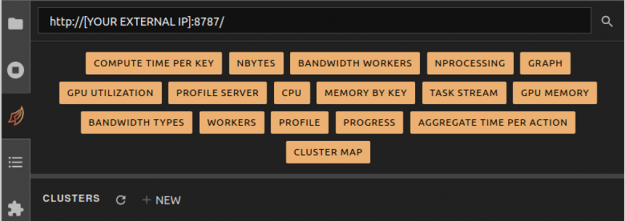
- Once the cluster is finished creating, you should see something like the screen below.
Running the next few cells will create a number of helper functions to help aggregate timings and scale worker counts, create some predefined data loading mechanisms for our medium and large NYC-Taxi datasets along with some pre-processing and data clean up, and create some simple visualization functions to let us explore the results.
ETL example
Most data scientists are probably aware that the choice of file format matters, but it’s not always clear how much or what the underlying trade off is. As a quick illustration, let’s look at the time required to read in ~150 million rows from CSV vs parquet data formats.
CSV
base_path = 'gcs://anaconda-public-data/nyc-taxi/csv'

with SimpleTimer() as timer_csv:
    df_csv_2014 = dask_cudf.read_csv(f'{base_path}/2014/yellow_*.csv', chunksize=25e6)
    df_csv_2014 = clean(df_csv_2014, remap, must_haves)
    df_csv_2014 = df_csv_2014.query(' and '.join(query_frags))

    with Dask.annotate(workers=set(workers)):
        df_csv_2014 = client.persist(collections=df_csv_2014)

    wait(df_csv_2014)

print(df_csv_2014.columns)
rows_csv = df_csv_2014.iloc[:,0].shape[0].compute()
print(f"CSV load took {timer_csv.elapsed/1e9} sec. For {rows_csv} rows of data => {rows_csv/(timer_csv.elapsed/1e9)} rows/sec")
On an eight GPU cluster this takes around 350 seconds, for ~155,500,000 rows.
Parquet
with SimpleTimer() as timer_parquet:
    df_parquet = dask_cudf.read_parquet(f'gs://anaconda-public-data/nyc-taxi/nyc.parquet', chunksize=25e6)
    df_parquet = clean(df_parquet, remap, must_haves)
    df_parquet = df_parquet.query(' and '.join(query_frags))

    with Dask.annotate(workers=set(workers)):
        df_parquet = client.persist(collections=df_parquet)

    wait(df_parquet)

print(df_parquet.columns)
rows_parquet = df_parquet.iloc[:,0].shape[0].compute()
print(f"Parquet load took {timer_parquet.elapsed/1e9} sec. For {rows_parquet} rows of data => {rows_parquet/(timer_parquet.elapsed/1e9)} rows/sec")
On the same eight GPU cluster, the parquet read takes around 98 seconds, for ~138,300,000 rows. A speedup of more than 3x over the CSV reads in terms of rows per second; for larger datasets this can result in a tremendous amount of time saved.
Multi-Node cuML training
Here, we’ll examine the process of training a Random Forest Regressor model across a set of workers in your cluster, examine the performance, and outline how we can scale up to more workers when necessary.
The performance sweep code goes through a fairly straightforward process.
- Calls the data loader, which reads and load-balances our dataset across Dask workers.
- Calls model.fit, ‘sample’ times, in either an X ~ y format for supervised models like RF, or just using X (KMeans, NN, etc..), and records the resulting timings.
- Calls model. predict, ‘sample’ times, for all rows in X, and records the resulting timings.
Two-Node performance
From the RAPIDS’ documentation: This distributed algorithm uses an embarrassingly-parallel approach. For a forest with N trees being built on w workers, each worker simply builds N/w trees on the data it has available locally. In many cases, partitioning the data so that each worker builds trees on a subset of the total dataset works well, but it generally requires the data to be well-shuffled in advance. Alternatively, callers can replicate all of the data across workers so that rf.fit receives w partitions, each containing the same data. This would produce results approximately identical to single-GPU fitting.
from cuml.dask.ensemble import RandomForestRegressor

rf_kwargs = {
    "workers": client.has_what().keys(),
    "n_estimators": 10,
    "max_depth": 6
}
rf_csv_path = f"./{out_prefix}_random_forest_classifier.csv"

benchmark_sweep(client=client, model=RandomForestRegressor,
                **benchmark_kwargs,
                out_path=rf_csv_path,
                response_dtype=np.int32,
                model_kwargs=rf_kwargs)

visualize_csv_data(rf_csv_path)
Running this, you’ll see the following:
Starting weak-scaling performance sweep for:
 model      : <class 'cuml.dask.ensemble.randomforestregressor.RandomForestRegressor'>
 data loader: <function taxi_parquet_data_loader at 0x7ff164a17790>.
Configuration
==========================
Worker counts             : [2]
Fit/Predict samples       : 5
Data load samples         : 1
- Max data fraction       : 1.00
 - Train                  : 1.00
 - Infer                  : 1.00
Model fit                 : X ~ y
- Response DType          : <class 'numpy.int32'>
Writing results to        : ./taxi_medium_random_forest_regression.csv
- Method                  : append


Sampling <1> load times with 2 workers.  With 12.5 percent of total data

100%|██████████| 1/1 [17:19<00:00, 1039.30s/it]
Finished loading <1>, samples, to <2> workers with a mean time of 1039.3022 sec.
Sweeping <class 'cuml.dask.ensemble.randomforestregressor.RandomForestRegressor'> 'fit' with <2> workers. Sampling  <5> times with 12.5 percent of total data.

100%|██████████| 5/5 [06:55<00:00, 83.04s/it]
Finished gathering <5>, 'fit' samples using <2>  workers, with a mean time of 83.0431 sec.
Sweeping <class 'cuml.dask.ensemble.randomforestregressor.RandomForestRegressor'> 'predict' with <2> workers. Sampling <5> times with 12.5 percent of total data.

100%|██████████| 5/5 [07:23<00:00, 88.60s/it]
Finished gathering <5>, 'predict' samples using <2>  workers, with a mean time of 88.6003 sec.


  hardware  n_workers     type     ci.low    ci.high
0        T4          2      fit  82.610233  83.476041
1        T4          2  predict  86.701627  90.498879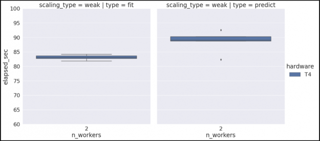
Note that if we wanted to check our algorithm performance for multiple hardware types, we could rerun the previous commands on a different cluster configuration, and since we’re set to append to our existing data set we would then see something similar to the graph below. (See the Vis and Analysis section of the notebook for more information).
Scaling up and out
At this point we’ve trained our random forest using two workers and collected some data; now let’s assume we want to scale up our workflow to support a larger dataset.
There are two possible scaling cases we need to consider, the first is that we want to scale our worker counts, and our Kubernetes cluster already has sufficient resources; in this case, all we need to do is tell our KubeCluster object to scale the cluster, and it will spin up additional worker pods and connect them to the scheduler.
n_workers = 16
cluster.scale(n_workers)
The second scenario is one where we don’t have sufficient Kubernetes resources to launch additional workers. In this case, we’ll need to go back to GKE and increase the size of our node pool before we can scale up our worker count. Once we’ve done that, we can go back and update our sweep configuration to run with four and eight workers, and kick off another run. Examining the results, we see the relatively flat profile that we would expect for a weak scaling run.
… SNIP …
  hardware  n_workers     type     ci.low    ci.high
0        T4          2      fit  82.610233  83.476041
2        T4          8  predict  21.372635  25.744045
3        T4         16      fit   3.417929   3.491950
6        T4         16  predict  17.952964  21.310312
8        T4          4  predict  45.985099  47.991526
9        T4          2  predict  86.701627  90.498879
10       T4          8      fit   8.470403   9.081820
11       T4          4      fit  30.791707  31.451253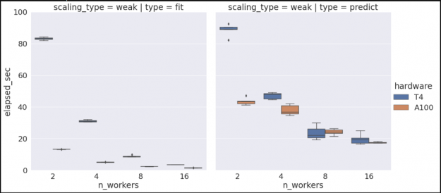
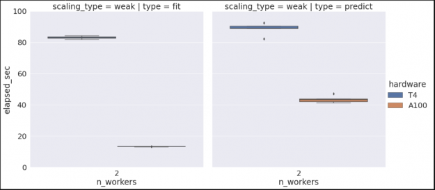
Similarly, if we want to gather additional scaling data for another hardware type, say V100’s, we can rebuild our cluster, selecting V100s instead of T4s, and re-run our performance sweeps to produce the following.
… SNIP …
  hardware  n_workers     type     ci.low    ci.high
1      A100          4  predict  36.307192  39.593791
2        T4          8  predict  21.372635  25.744045
3        T4         16      fit   3.417929   3.491950
4      A100         16      fit   1.438821   1.541184
7      A100          8  predict  23.161591  25.073527
9        T4          8      fit   8.470403   9.081820
10     A100          4      fit   5.009861   5.124773
11       T4          4      fit  30.791707  31.451253
13       T4          2      fit  82.610233  83.476041
14     A100          2      fit  13.178733  13.259799
15     A100          2  predict  42.331923  44.573160
17     A100         16  predict  17.292678  17.742979
19       T4         16  predict  17.952964  21.310312
21     A100          8      fit   2.302896   2.337939
22       T4          4  predict  45.985099  47.991526
23       T4          2  predict  86.701627  90.498879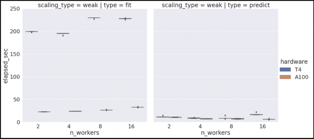
XGBoost performance
Following similar steps, we can evaluate cluster performance for all our other algorithms, including XGBoost. The following example is trained on a subset of the much larger ‘mortgage’ dataset, which is available here. Note that because this dataset is not publicly hosted on GCP, some additional steps are required to pull the data, push to a private GCP bucket, convert the dataset to Parquet. The setup required for GCP/GKE is covered in the optional portion of the ‘Kubernetes on GKE’ section of this document; the scripts for converting the mortgage dataset to parquet can be found here.
In addition to the steps described above, we will also utilize the RAPIDS Forest Inference Library (FIL) framework for accelerated inference of our trained XGBoost model. The process for this is somewhat different from what occurs with RandomForest. After training our initial XGBoost model is fit, we will save the model to a centralized GCP bucket, and subsequently instantiate the model as a FIL object on each of our available workers. Once that step is completed, we can perform FIL based inference locally on each worker for its portion of the dataset.
Conclusion
Congratulations! At this point you’ve gone through the process of spinning up a Dask cluster in GKE, loaded a substantial dataset, performed distributed training using multiple nodes and GPUs, and built familiarity with the Dask ecosystem and monitoring tools for Jupyter.
Going forward, this should provide you with a basic template for utilizing Dask, RAPIDS, and XGboost with your own datasets to build and evaluate your workflow in Kubernetes.
For more information about the technologies we’ve used, such as RAPIDS, Dask, and Kubernetes, check out the links below.
