
It is well-known that GPUs are the typical go-to solution for large machine learning (ML) applications, but what if GPUs were applied to earlier stages of the data-to-AI pipeline?
For example, it would be simpler if you did not have to switch out cluster configurations for each pipeline processing stage. You might still have some questions:
- Would this be practical from a cost perspective?
- Could you still meet SLAs on a data-processing time budget for some near-real-time processing?
- How difficult is it to optimize these GPU clusters?
- If you optimized the configuration for one stage, would the same work for other stages?
At AT&T, these questions arose when our data teams were working to manage cloud costs while balancing simplicity at scale. We also observed that many of our data engineers and scientist colleagues were not aware of GPUs being an effective and efficient infrastructure on which to run more mundane ETL and feature engineering stages.
It was also not clear what the relative performance could be of CPU compared to GPU configurations. Our goal at AT&T was to run a few typical configuration examples to understand the difference.
In this post, we share our data pipeline analysis in terms of speed, cost, and full pipeline simplicity. We also provide insights on design considerations and explain how we optimized the performance and price of our GPU cluster. The optimization came from using the RAPIDS accelerator for Apache Spark, an open-source library that enables GPU-accelerated ETL and feature engineering.
SPOILER ALERT: We were pleasantly surprised that, at least for the examples examined, the use of GPUs for each pipeline stage proved to be faster, cheaper, and simpler!
Use cases
Data-to-AI pipelines include multiple stages of batch processing:
- Data preparation or federation
- Transformation
- Feature engineering
- Data extraction
Batch processing involves processing a large volume of data containing trillions of records. Batch processing jobs are generally optimized for either cost or performance depending on the SLA for that use case.
A good example of a batch processing job optimized for cost is creating features from call records, which go on to be used to train an ML model. On the other hand, a real-time, inference use case to detect fraud is optimized for performance. GPUs are often overlooked and considered to be expensive for these batch-processing stages of AI/ML pipelines.
These batch processing jobs often involve large joins, aggregation, ranking, and transformation operations. As you can imagine, AT&T has many data and AI use cases that involve batch processing:
- Network planning and optimization
- Fraud
- Sales and marketing
- Tax
Depending on the use case, these pipelines can use NVIDIA GPUs and RAPIDS Accelerator for Apache Spark to optimize costs or improve performance.
For this analysis, we look at a couple of data-to-AI pipelines. The first uses feature engineering of call records for a marketing use case, and the second use case carries out an ETL transformation of a complex tax dataset.
Speeding up feature engineering and transformation with GPUs
Efficiently scaling data-to-AI pipelines remains a need for data teams. High-cost pipelines are processing hundreds of terabytes to petabytes of data on a monthly, weekly, or even daily basis.
When examining efficiency, it is important to identify optimization opportunities across all ETL and feature engineering stages and then compare speed, cost, and pipeline simplicity.
For our data pipeline analysis, we compared three options:
- Various CPU-based Spark cluster solutions
- RAPIDS accelerator for Apache Spark on a Spark GPU cluster
- An Apache Spark CPU cluster using Databricks’ newly released Photon engine
To gauge how far we were from the optimum cost, we compared a bare-bone VM solution using AT&T’s open-sourced GS-lite solution that enables you to write SQL that then compiles to C++.
As mentioned earlier, after optimizing each solution, we discovered that the RAPIDS accelerator for Apache Spark running on a GPU cluster, had the best overall speed, cost, and design simplicity trade-off.
In the following sections, we discuss the chosen optimizations and design considerations for each.
Design considerations for optimizing the AI/ML pipeline solution
To compare the performance of the three potential solutions, we carried out two experiments, one for each of the selected use cases. For each, we optimized different parameters to gain insight into how speed, cost, and design are affected.
Example 1: Optimizing simple group by aggregations for the call-records use case
For the first feature engineering example, we chose to create features from call-record datasets containing close to three trillion records (rows) a month (Table 1). This data preprocessing use case is a fundamental building block in several sales and marketing AI pipelines, such as customer segmentation, predicting customer churn, and anticipating customer trends and sentiments. There were various data transformations in this use case, but many of them involved simple “group by” aggregations such as the following, for which we wanted to optimize the processing.
res=spark.sql("""
Select DataHour, dev_id,
    sum(fromsubbytes) as fromsubbytes_total,
    sum(tosubbytes) as tosubbytes_total,
From df
Group By DataHour, dev_id
""")
Accessing insights from data and carrying out data analysis is still one of the biggest pain points for many enterprises. This is not because of lack of data, but because the amount of time spent on data preparation and analysis is still an impediment to data engineers and data scientists.
Here are some of the key infrastructure challenges in this preprocessing example:
- Query execution on CPU cluster takes too long, leading to timeout issues.
- The compute cost is expensive.
| Days | # of Rows | Size (Bytes) |
| 1 | ~110 Billion | >2 TB |
| 7 | ~800 Billion | ~16 TB |
| 30 | ~3 Trillion | ~70 TB |
Also, this call-records use case had an extra dimension of experimentation in terms of compression types. The data was arriving from the network edge to the cloud with some form of compression that we could specify and evaluate tradeoffs for. We thus experimented with several compression schemes, including txt/gzip, Parquet/Z standard, and Parquet/Snappy.
The Z-standard compression had the smallest file size (about half in this case). As we show later, we found better speed/cost tradeoffs with Parquet/Snappy.
Next, we considered the type of cluster with regard to the number of cores per VM, number of VMs, the allocation of worker nodes, and whether to use a CPU or GPU.
- For CPU clusters, we chose the lowest number of cores that could handle the workload, that is, the lowest number of VMs and workers to prevent an over-allocation of resources.
- For GPUs, we used the RAPIDS Accelerator tuning guide [spark-rapids-tuning], which provides sizing recommendations with regard to concurrent tasks per executor, maxPartitionBytes, shuffle partitions, and concurrent GPU tasks.
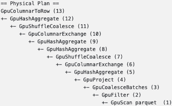
One goal after implementing the data processing on the GPU was to ensure that all key feature engineering steps remained on the GPU (Figure 1).
Example 2: Optimizing multiple ETL and feature creation stages for the tax dataset
The use case for Example 2 allowed us to compare many different transformations and processing stages for ETL, feature creation, and AI. Each stage had different record volume sizes (Figure 2).
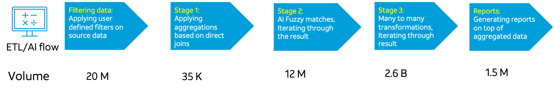
This ETL pipeline with multiple stages is a common bottleneck in enterprises where data lives in silos. Most often massive data processing requires querying and joining data from two or more data sources using fuzzy logic. As you can see from Figure 2, even though we started only with 20 million rows of data, the data volume grew exponentially as we moved through the data processing stages.
As in Example 1, the design considerations were the number of cores per VM, number of VMs, and the allocation of worker nodes, when comparing CPUs and GPUs.
Results
After trying different core, worker, and cluster configurations for the use cases shown in examples 1 and 2, we collected the results. We ensured that any particular ETL job finished within the allocated time to keep up with the data input data rate. The best approach in both had the lowest cost and highest simplicity.
Example 1 results
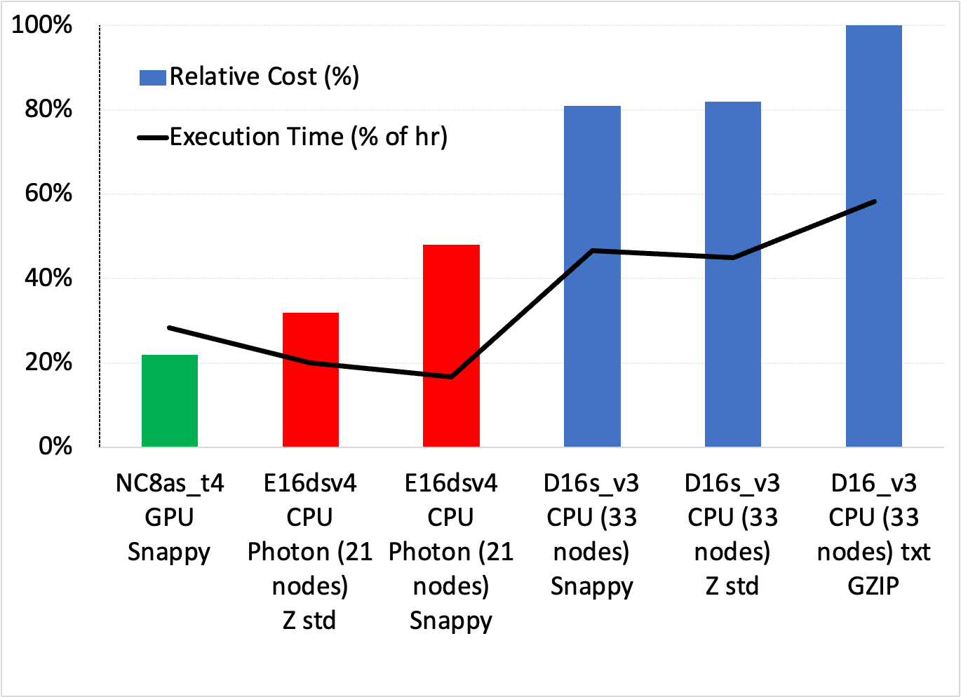
Figure 3 shows the cost/speed tradeoffs across a range of setups for simple group by aggregations in the call records use case. You can make several observations:
- The lowest cost and simplest solution is using the GPU cluster with Snappy compression, being ~33% cheaper than the lowest-cost Photon solution and close to half the cost of the fastest Photon solution.
- All standard Databricks clusters performed worse on both cost and execution time. Photon was the best CPU solution.
While not shown in Figure 3, the GS-lite solution was actually the cheapest, needing only two VMs.
Example 2 results
Like Example 1, we tried several CPU and GPU cluster configurations for the five ETL and AI data processing stages with the Databricks 10.4 LTS ML runtime. Table 2 shows the resulting best configurations.
| Configuration | CPU | GPU |
| Worker type | Standard_D13_v2 56 GB memory, 8 cores, min workers 8, max workers 12 | Standard_NC8as_T4_v3 56 GB memory, 1 GPU, min workers 2, max workers 16 |
| Driver type | Standard_D13_v2 56 GB memory, 8 cores | Standard_NC8as_T4_v3 56 GB memory, 1 GPU |
These configurations yielded the relative cost and execution time (speed) performances favoring GPUs (Figure 4).
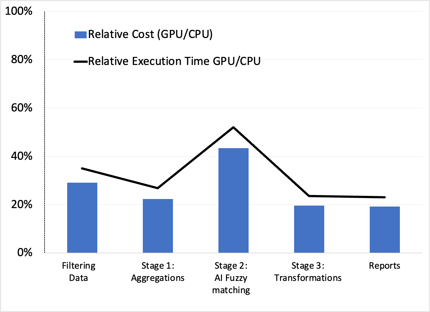
While not shown here, we confirmed that the next stages of the AI pipeline in Example 1, which used XGBoost modeling, also benefited from GPUs and RAPIDS Accelerator for Apache Spark. This confirms that GPUs could be the best end-to-end solution.
Conclusion
While not exhaustive of all AT&T’s data and AI pipelines, it appears that GPU-based pipelines were beneficial in all examples examined. In these cases, we were able to cut down the time for data preparation, model training, and optimization. This resulted in spending less money with a simpler design, as there was no configuration switching across stages.
We encourage you to experiment with your own data to AI pipelines, especially if you’re already using GPUs for AI/ML training. You may also find that GPUs are your “go-to,” simpler, faster, and cheaper solution!
Interested in learning more about these use cases and experiments, or getting tips on how to cut down your data processing time with the RAPIDS Accelerator for Apache Spark? Register for the free AT&T GTC session, How AT&T Supercharged their Data Science Efforts.
