The NVIDIA Vision Programming Interface (VPI) is a software library that provides a set of computer-vision and image-processing algorithms. The implementations of these algorithms are accelerated on different hardware engines available on NVIDIA Jetson embedded computers or discrete GPUs.

In this post, we show you how to run the Temporal Noise Reduction (TNR) sample application on the Jetson product family. For more information, see the VPI – Vision Programming Interface documentation.
Setting up VPI on a Jetson device
While setting up a Jetson device through the SDK Manager, make sure to have the Jetson SDK components box checked. VPI is then installed as the device is flashed. For more information about installation, see NVIDIA SDK Manager.
When the installation is completed, VPI can be found under the following path:
/opt/nvidia/vpi1/
To validate the environment has been set correctly, copy VPI sample applications into your home directory and then build the TNR sample.
$ vpi1_install_samples.sh $HOME
$ cd $HOME/NVIDIA_VPI–samples/09-tnr
$ cmake .
$ make
VPI is also supported on x86 machines running discrete GPUs. For more information, see Installation in the VPI – Vision Programming Interface documentation.
TNR sample application
VPI provides a set of CV algorithms that leverage multiple backends to use the available compute resources of the device efficiently. TNR is a noise-reduction method commonly used in computer-vision applications running on a Jetson device. This post uses the TNR sample application to demonstrate how you can go about implementing your own application using some key concepts and components in VPI.
We cover the following topics in this post:
- Creating the necessary elements to build a VPI pipeline
- Understanding how the interoperability with OpenCV takes place
- Submitting processing tasks to a stream
- Synchronizing the tasks in a stream
- Locking an image buffer so that it is accessible from the CPU
The TNR sample can be found in the following path:
$HOME/NVIDIA_VPI–samples/09-tnr/main.cpp
For more information about the sample application and algorithm, see the following resources:
Algorithm versions and backend support
The hardware engines are named backends in VPI. These backends enable you to offload parallelizable processing stages and accelerate the application by using the available system-level parallelism inherent to the Jetson devices. The backends are CPU, CUDA (GPU), PVA, and VIC. The exact availability of a specific backend engine depends on the Jetson platform onto which the application is deployed. For more information about the available algorithms, backend support, and backend availability on specific platforms, see Algorithms.
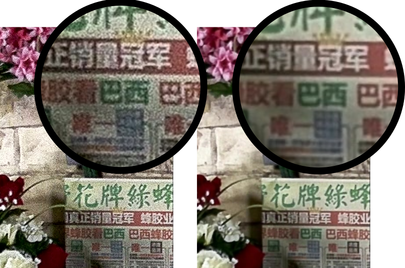
VPI currently provides two different implementations for TNR, which each suit different scenarios and requirements. These versions employ a combination of bilateral filtering for smoothing flat regions while preserving edges, and temporal infinite impulse response (IIR) filtering with a motion detector to tackle temporal noise across frames.
- VPI_TNR_V2—This version offers a lighter noise reduction when compared to VPI_TNR_V3 and a certain degree of configurability, namely lighting conditions can be adjusted to better fit a given scenario. This version has a reduced computational demand, which translates into speed. It suits use cases where execution time is more important than the noise reduction quality.
- VPI_TNR_V3—For use cases where a noise reduction with better quality is needed. With this variant, you should expect an increase in computational demand in comparison to VPI_TNR_V2. On top of this, configurability is further extended. It is recommended for challenging low-light scenarios.
- VPI_TNR_DEFAULT—Instead of specifying the exact version, you can use the default value, which picks the version with the strongest noise reduction supported by the given backend.
Another criterion to consider when deciding which algorithm version suits your use case is its support across different backends and devices. The following table summarizes TNR support.
| Backend/Device | Jetson Nano series | Jetson TX2 series | Jetson Xavier series |
| CUDA (GPU) | VPI_TNR_V3 | VPI_TNR_V3 | VPI_TNR_V3 |
| VIC | VPI_TNR_V2 | VPI_TNR_V2 | VPI_TNR_V2 and VPI_TNR_V3 |
| CPU | Not yet supported | Not yet supported | Not yet supported |
| PVA | Backend not available | Backend not available | Not applicable |
Both VPI_TNR_V2 and VPI_TNR_V3 enable tuning by allowing you to explicitly set the lighting conditions of the scene you are capturing. This is important in the context of low-light scenes or streams captured with high-gain that may contain higher noise levels, and therefore demand a higher level of noise reduction.
Higher strength levels may affect the number of details in textured regions of the frames, smoothing them out. Another side effect is ghosting in scenes where there are fast-moving objects. The supported scene lighting conditions vary in terms of type (indoor, outdoor) and intensity (low, medium, and high), as summarized in the following table.
| Scene | Description |
| VPI_TNR_PRESET_OUTDOOR_LOW_LIGHT | Outdoor scenes with poor lighting conditions, leading to high noise. |
| VPI_TNR_PRESET_OUTDOOR_MEDIUM_LIGHT | Outdoor scenes with sufficient lighting but still with some noise. |
| VPI_TNR_PRESET_OUTDOOR_HIGH_LIGHT | Outdoor scenes with good lighting conditions and less noise. |
| VPI_TNR_PRESET_INDOOR_LOW_LIGHT | Indoor scenes with poor lighting conditions. |
| VPI_TNR_PRESET_INDOOR_MEDIUM_LIGHT | Indoor scenes with sufficient lighting. |
| VPI_TNR_PRESET_INDOOR_HIGH_LIGHT | Indoor scenes with good lighting. |
With the different versions and associated lighting conditions presets, you can adjust the TNR algorithm to the specifics of your use case. This can be further customized with the so-called strength factor. It is a float parameter ranging from 0 to 1, where larger values correspond to increased denoizing strength.
VPI applications
One of the key aspects about VPI is how it manages and coordinates resources required for running an application among different backends. With VPI, it is possible to avoid wasteful memory copies between processing stages. Another mechanism enforced by VPI for an efficient memory management is memory wrapping at its interfaces.
Taking advantage of all the memory management features of VPI depends on how your code is structured. The best practice is seeing your code as a three-stage workflow:
- Initialization
- Processing loop
- Cleanup
Most of the memory allocation should happen during the initialization phase. This is particularly important in the context of embedded applications that operate on devices with constraints in terms of available resources. On top of that, memory management can be done more efficiently and carefully to avoid possible memory leakage.
A good practice in VPI is specifying the backends on which a piece of memory is used. On that note, subscribing your VPI objects only to the set of backends that you need guarantees you the most efficient path for memory as the pipeline flows between those backends.
The processing loop is where the processing pipeline gets executed. Imagine an application iterating over a video file with hundreds of individual frames. The main loop would be primarily in charge of executing the needed transformations on the pixel information to achieve the desired outcome of the given computer-vision task.
Lastly, the cleanup phase handles all the necessary freeing and deallocation of the resources that have been used during the execution of the task. Sticking to this paradigm enables VPI to use the most efficient processing pipeline possible and helps you adhere to good coding practices.
Interfacing with OpenCV
The interoperability of VPI with OpenCV is a distinct feature of the library. If you’re familiar with OpenCV, you can easily integrate VPI with your workflow or extend existing data pipelines to better use the hardware acceleration provided by VPI.
This is demonstrated in the TNR sample through the following utility function, which wraps the input video frames captured using OpenCV into a VPI image object.
  69 // Utility function to wrap a cv::Mat into a VPIImage
  70 static VPIImage ToVPIImage(VPIImage image, const cv::Mat &frame)
  71 {
  72     if (image == nullptr)
  73     {
  74         // Create a VPIImage that wraps the frame
  75         CHECK_STATUS(vpiImageCreateOpenCVMatWrapper(frame, 0, &image));
  76     }
  77     else
  78     {
  79         // reuse existing VPIImage wrapper to wrap the new frame.
  80         CHECK_STATUS(vpiImageSetWrappedOpenCVMat(image, frame));
  81     }
  82     return image;
  83 }
Start by digging a bit deeper into the function described earlier. It is meant to wrap a OpenCV matrix (cv::Mat) object into a VPI image object (VPIImage). To contextualize, VPI images are essentially any 2D data structures that can be described in terms of their width, height, and format. Even though it is intuitive to see image data as a VPIImage object, its usage can also be extended to other types of data, such as 2D vector fields and heat maps.
The utility wrapping function invokes two other functions that pertain to the VPI OpenCVInterop.hpp module, which aims to provide useful infrastructure to integrate OpenCV-based code with VPI.
- vpiImageCreateOpenCVMatWrapper—An overloaded function that wraps a
cv:Matobject intoVPIImagein two different flavors. The first tries to infer the format directly from the input type (following specific rules), while the second takes an explicit format as one of its arguments. - vpiImageSetWrappedOpenCVMat—Reuses a wrapper defined for a specific
cv::Matobject to wrap a new incomingcv::Matobject. The point here is avoiding the memory allocation that incurs from creating a wrapper in the first place, which is therefore more efficient. The incomingcv::Matobject must present the same characteristics (format and dimensions) as the original one used at the creation time.
Stream creation
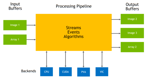
The main function captures the relevant steps for setting up a VPI pipeline to get the work done. The definition of a pipeline is straightforward and rather intuitive. In VPI, pipelines are a composition of one or multiple streams of data that flow through different processing stages.
Figure 1 shows a pipeline and its building blocks (streams, buffers, algorithms, and so on) in a generic way. For the sake of simplicity, some components have been omitted.
The purpose of a stream is to enforce a queued sequence of steps that the data needs to go through to fulfill a specific computer-vision task. Those steps may encompass pre– or post-processing of the data or even full-fledged algorithms such as TNR. Figure 2 shows an example of a VPIStream object.
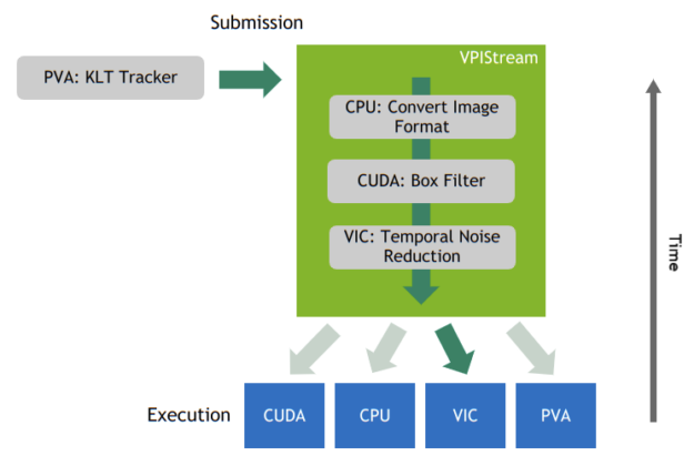
VPI accommodates for a varying range of pipeline complexity. You can implement a simple pipeline with a single stream or, alternatively, have a more complex implementation with several parallel streams with different stages offloaded to different compute backends. This is a powerful feature of the API as it enables you to gain even more control over the system-level parallelism offered by the Jetson devices.
The following code example demonstrates how the stream is created in the TNR sample.
 143        VPIStream stream;
 144         // PVA backend doesn't have currently Convert Image Format algorithm.
 145         // Use the CUDA backend to do that.
 146         CHECK_STATUS(vpiStreamCreate(VPI_BACKEND_CUDA | backend, &stream));
A selection of backends is being passed onto the stream. This is an optional step. Using a value of zero would enable all available backends. However, assigning a specific set of backends is a recommended practice as it helps to optimize memory allocation.
TNR payload
Payloads are essentially temporary resources that are required during the execution of a pipeline. For example, a payload could be an intermediate memory buffer that stores data traded between subsequent stages of a stream. Many algorithms, including TNR, require the explicit creation of a payload, which can be achieved as follows.
 172         // Create a TNR payload configured to process NV12
 173         // frames under outdoor low-light scenarios.
 174        VPIPayload tnr;
 175         CHECK_STATUS(vpiCreateTemporalNoiseReduction(backend, w, h, VPI_IMAGE_FORMAT_NV12_ER, VPI_TNR_DEFAULT,
 176                                                     VPI_TNR_PRESET_INDOOR_LOW_LIGHT, 1, &tnr));
For the TNR payload, provide the following arguments:
- Image dimensions (width and height)
- Backend
- Format of the image data (currently, only NV12 is supported)
- TNR algorithm version
- Lighting conditions
- Noise reduction strength
- Reference to the algorithm payload
Ultimately, the function creates a payload and ties it to the assigned backend.
Image buffers
Besides the stream and payload creation, the image buffers required by the VPI algorithm also must be created. In TNR, a combination of bilateral and IIR filters is used and so three different buffers are required; namely, the current and previous image input and the image output.
The image buffers can be created as follows:
167        VPIImage imgPrevious, imgCurrent, imgOutput;
168         CHECK_STATUS(vpiImageCreate(w, h,VPI_IMAGE_FORMAT_NV12_ER, 0, &imgPrevious));
169         CHECK_STATUS(vpiImageCreate(w, h,VPI_IMAGE_FORMAT_NV12_ER, 0, &imgCurrent));
170         CHECK_STATUS(vpiImageCreate(w, h,VPI_IMAGE_FORMAT_NV12_ER, 0, &imgOutput));
This creates empty buffers with the following assigned characteristics:
- Image dimensions (width and height)
- Format (as required by the algorithm)
- Image flags (currently used to assign the backends)
- Pointer to the variable where the
VPIImagehandle for the created image is returned
Stream processing
With the building blocks already in place, you can move on to the main processing loop, where the execution of the noise reduction algorithm takes place. On the TNR sample, the loop is iterating each individual frame from a video file and performing the necessary sequential steps to achieve the desired outcome.
The first step, as the frame is collected from the video, is to wrap it into a VPIImage object using the utility function described earlier.
186 frameBGR = ToVPIImage(frameBGR, cvFrame);
As the wrapping is completed, VPI is now able to operate on the pixel data in the VPIImage object. Because TNR requires the frame to be in NV12 format, a conversion step is required.
188             // First convert it to NV12
189             CHECK_STATUS(vpiSubmitConvertImageFormat(stream,VPI_BACKEND_CUDA, frameBGR, imgCurrent, NULL));
At this stage, the specific task of converting the image is being associated with the stream instantiated previously. On top of that, the task is being set to perform on the GPU. The image buffer for the input frame as well as data that has just been wrapped from the cv::Mat object are used for that.
As the format conversion is completed, the input buffer can be passed to the TNR algorithm for processing.
191             // Apply TNR
192             // For first frame, you must pass nullptr as the previous frame, this resets the internal
193             // state.
194             CHECK_STATUS(vpiSubmitTemporalNoiseReduction(stream, 0, tnr, curFrame == 1 ? nullptr : imgPrevious,
195                                                          imgCurrent, imgOutput));
196
For invoking the TNR algorithm, set the following parameters:
- The stream with which the algorithm is associated
- The backend
- The algorithm payload, as the one instantiated previously
- Image buffers: previous and current inputs and output
At the first iteration (curFrame == 1), there is no valid previous image on the buffer and a null pointer is passed instead. For the following iterations, the buffer is populated accordingly. After the execution of the TNR algorithm, the output buffer can then be converted back from NV12 to its previous BGR format.
197             // Convert output back to BGR
198             CHECK_STATUS(vpiSubmitConvertImageFormat(stream,VPI_BACKEND_CUDA, imgOutput, frameBGR, NULL));
At this point, it is crucial to mention that VPI enforces a non-blocking asynchronous paradigm to the stream stages. This is essential for a smooth and efficient orchestration of workloads distributed among different coprocessors as backends. For further steps, make sure that all activity issued to the stream is finished before proceeding. That’s when the synchronization function comes in handy.
199 CHECK_STATUS(vpiStreamSync(stream));
VPI now makes sure that every ongoing activity associated with the stream is finished before moving on to the next stages of the pipeline. When synchronization completes, the frame is ready and available in the output buffer connected to the specified backend. To be able to write it out to the output video stream—in this case, a file, the image must be locked so that the buffer is made available to the CPU.
This explains why synchronizing right before locking the frame is a key step to avoid problems with processing. Because VPI operates asynchronously, it might happen that, without synchronization, the buffer is locked before the previous stages complete. The results here would be unpredictable.
 201             // Now add it to the output video stream
 202            VPIImageData imgdata;
 203             CHECK_STATUS(vpiImageLock(frameBGR,VPI_LOCK_READ, &imgdata));
 204
 205             cv::Mat outFrame;
 206             CHECK_STATUS(vpiImageDataExportOpenCVMat(imgdata, &outFrame));
 207             outVideo << outFrame;
 208
 209             CHECK_STATUS(vpiImageUnlock(frameBGR));
As you can see, the locked buffer is at the CPU’s disposal for further use. The lock is set as a read-only and then the image buffer gets mapped to the CPU. While locked, VPI cannot work on the buffer. After the CPU provides the output frame to the video encoder, the buffer can be unlocked and further used by VPI.
VPI dataflow
The TNR sample application can be summarized as the following dataflow. Other minor steps are also an integral part of the application but for the sake of simplicity, only the macro steps have been included in Figure 3.

- The input frame is collected from a video stream or file. OpenCV has been used for this purpose.
- The necessary VPI elements are instantiated: a single stream, a TNR algorithm payload, and image buffers for previous and current input and output images.
- The input frame is wrapped into a
VPIImagebuffer. - The pixel data on the buffers is converted to NV12 so that the TNR algorithm can process it. It is brought back to its original format as the algorithm completes execution.
- The image buffer is locked so that the data is accessible to the CPU. After providing the image to the video output, the buffer can be unlocked and VPI can further work on it.
Summary
In this post, we showed you how to run the TNR sample application on the Jetson product family. For more information, see VPI – Vision Programming Interface Documentation.
