This guest post by Daniel Armyr and Dan Doherty from MathWorks describes how you can use MATLAB to support your development of CUDA C and C++ kernels. You will need MATLAB, Parallel Computing Toolbox™, and Image Processing Toolbox™ to run the code. You can request a trial of these products. For a more detailed description of this workflow, refer to the MATLAB for CUDA Programmers webinar and associated demo files.
NVIDIA GPUs are becoming increasingly popular for large-scale computations in image processing, financial modeling, signal processing, and other applications—largely due to their highly parallel architecture and high computational throughput. The CUDA programming model lets programmers exploit the full power of this architecture by providing fine-grained control over how computations are divided among parallel threads and executed on the device. The resulting algorithms often run much faster than traditional code written for the CPU.
While algorithms written for the GPU are often much faster, the process of building a framework for developing and testing them can be time-consuming. Many programmers write CUDA kernels integrated into C or Fortran programs for production. For this reason, they often use these languages to iterate on and test their kernels, which requires writing significant amounts of “glue code” for tasks such as transferring data to the GPU, managing GPU memory, initializing and launching CUDA kernels, and visualizing kernel outputs. This glue code is time-consuming to write and may be difficult to change if, for example, you want to run the kernel on different input data or visualize kernel outputs using a different type of plot.
Using an image white balancing example, this article describes how MATLAB® supports CUDA kernel development by providing a language and development environment for quickly evaluating kernels, analyzing and visualizing kernel results, and writing test harnesses to validate kernel results.
Image White Balancing Example
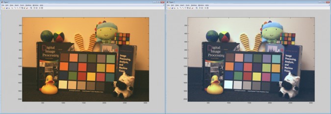
White balancing is a technique used to adjust the colors in an image so that the image does not have a reddish or bluish tint. Suppose you want to write a white balance routine in CUDA C for integration into a larger C program. Before writing any C code, it’s useful to explore the algorithm, investigate different algorithmic approaches, and develop a working prototype. We do this in MATLAB using the following code.
function imageData = whitebalance(imageData)
% WHITEBALANCE forces the average image color to be gray.
% Copyright 2013 The MathWorks, Inc.

% Find the average values for each channel.
avg_rgb = mean(mean(imageData));

% Find the average gray value and compute the scaling
% factor.
factors = max(mean(avg_rgb), 128)./avg_rgb;

% Adjust the image to the new gray value.
imageData(:,:,1) = uint8(imageData(:,:,1)*factors(1));
imageData(:,:,2) = uint8(imageData(:,:,2)*factors(2));
imageData(:,:,3) = uint8(imageData(:,:,3)*factors(3));
This code computes the average amount of each color present in the input image and then applies scaling factors to ensure that the output image has an equal amount of each color. Notice that, with MATLAB, developing the algorithm takes just five lines of code—far fewer than it would take in C or Fortran. One reason is that MATLAB is a high-level, interpreted language that automates administrative tasks such as declaring variables and allocating memory. Another is that MATLAB includes thousands of built-in math, engineering, and plotting functions and can be extended with domain-specific algorithms in signal and image processing, computational finance, communications, and other areas. We call the MATLAB white balance algorithm using an input image that includes a Gretag Macbeth color chart, which is commonly used to calibrate cameras. We then visualize the output using the imshow command in Image Processing Toolbox™.
adjustedImage = whitebalance(imagedata);
imshow(adjustedImage);
The algorithm removes the reddish tint from the original image (Figure 1).
This working MATLAB implementation will serve as a reference as we develop and test CUDA kernels for the white balance algorithm.
Exploring MATLAB Code and Implementing Portions in CUDA C
We ultimately want to implement the white balance algorithm in C, with each computational step written as a CUDA kernel. Before getting started with CUDA, we use the MATLAB white balance code to explore the algorithm and decide how to break it into kernels. We begin by using the MATLAB Profiler to see how long each section of code takes to execute. The profiler shows the bottleneck areas where we need to spend extra effort to develop efficient CUDA kernels. We launch the MATLAB Profiler using the Run and Time button on the MATLAB desktop (Figure 2).
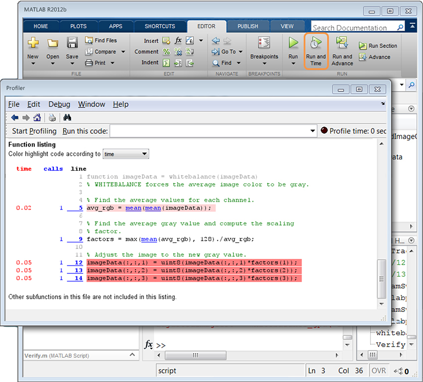
We see that the last three lines of code take 0.15 seconds to run, making this the most time-consuming section of the algorithm. This code scales every pixel value in the image, which is a naturally parallel operation that can be accelerated significantly on the GPU. We reimplement this code in CUDA C/C++ using the following kernel function.
// Copyright 2013 The MathWorks, Inc.
__global__
void applyScaleFactors( unsigned char * const out,
    const unsigned char * const in, const double *factor,
    unsigned int const numRows, unsigned int const numCols )
{
    // Work out which pixel we are working on.
    const int rowIdx = blockIdx.x * blockDim.x + threadIdx.x;
    const int colIdx = blockIdx.y;
    const int sliceIdx = threadIdx.z;

    // Check this thread isn't off the image
    if( rowIdx >= numRows ) return;

    // Compute the index of my element
    const unsigned int linearIdx = rowIdx + colIdx*numRows +
        sliceIdx*numRows*numCols;

    // Scale the value with the appropriate factor
    double result = (double)in[linearIdx]*factor[sliceIdx];

    // Cap our values to the interval [0,255]
    result = min(255.0,result);

    // Write the value to global memory.
    out[linearIdx] =  (unsigned char)rint(result);
}
Before writing kernels for the other computational steps in the white balance algorithm, we will transition back to MATLAB to run and test this kernel to make sure that it runs properly and gives correct results.
Evaluating the CUDA Kernel in MATLAB
To load the kernel into MATLAB, we specify paths to the compiled PTX file and source code (see the complete demo source code for how to invoke the nvcc compiler from Matlab code).
kernel = parallel.gpu.CUDAKernel( 'applyScaleFactorsKernel.ptx', ...
  'applyScaleFactorsKernel.cu' );
Once the kernel loads we must complete a few setup tasks before we can launch it, such as initializing return data and setting the sizes of the thread blocks and grid. The kernel can then be used just like any other MATLAB function, except that we launch the kernel using the feval command, with the following syntax.
[outArguments] = feval(kernelName, inArguments)
We replace the last three lines of code in our MATLAB white balance algorithm with code that loads and launches the kernel. The updated white balance routine (whitebalance_gpu.m) follows.
function adjustedImage = whitebalance_gpu(imageData)
% WHITEBALANCE_GPU forces the average image color to be gray.
% Copyright 2013 The MathWorks, Inc.

% Find the average values for each channel.
avg_rgb = mean(mean(imageData));

% Find the average gray value and compute the scaling factor.
factors = max(mean(avg_rgb), 128)./avg_rgb;

% Load the kernel
kernel = parallel.gpu.CUDAKernel('applyScaleFactors.ptxw64', ...
    'applyScaleFactors.cu' );

% Set up the threads
[nRows, nCols, ~] = size(imageData);
blockSize = 256;
kernel.ThreadBlockSize = [blockSize, 1, 3];
kernel.GridSize = [ceil(nRows/blockSize), nCols];

% Copy our image data to the GPU
imageDataGPU = gpuArray( imageData );

% Allocate and initialize return data, directly on the GPU
adjustedImageGPU = gpuArray.zeros( size(imageDataGPU), 'uint8');

% Apply the kernel to scale the color values
adjustedImageGPU = feval( kernel, adjustedImageGPU, imageDataGPU, ...
    factors, nRows, nCols );

% Copy data from the GPU back to main memory.
adjustedImage = gather( adjustedImageGPU );
Notice the relative ease of calling CUDA kernels from MATLAB. Each task, such as transferring data to the GPU, initializing return data, and launching the kernel, is performed using a single line of MATLAB code. Furthermore, the code is robust in that we can run the kernel for different sized images without updating the code. In lower-level languages like C or Fortran, the process of moving the data to the GPU, managing memory, and launching CUDA kernels requires more coding. We feel that the code is not only more difficult to write, but also more difficult for other developers and project collaborators to understand and modify for their own purposes.
Using the MATLAB Prototype Code as a Test Harness
Now that we have integrated our kernel into MATLAB, we test whether the results are correct by comparing the original MATLAB implementation of the white balance algorithm (whitebalance.m) with the new version that incorporates the kernel (whitebalance_gpu.m)
%% Load some input data
load ('imageData.mat')

%% Run the data through the two implementations
adjustedImageCPU = whitebalance(imageData);
adjustedImageGPU = whitebalance_gpu(imageData);

%% Visualize the results and their difference
subplot(1,2,1); imshow(adjustedImageCPU); title('CUDA Implementation');
subplot(1,2,2); imshow(adjustedImageGPU); title('MATLAB Implementation');

difference = double(adjustedImageCPU(:) - adjustedImageGPU(:));
msgbox(['The norm of the difference is: ' num2str(norm(difference))]);
We see that the output images appear identical, providing visual validation that the kernel is working properly (Figure 3). We also calculate the norm of the difference of the output images to be zero, which validates the kernel numerically.

We could easily use this test harness to test the kernel for additional input images with different characteristics. We could also develop more sophisticated test harnesses to do more detailed post processing or to automate testing.
Incrementally Developing Additional CUDA Kernels
So far, we have reimplemented one part of the white balance algorithm in CUDA. We ultimately want the entire algorithm written using CUDA kernels, since the major computational steps are parallelizable and good candidates for the GPU. Performing the entire computation on the GPU would also reduce the overhead associated with transferring data between the CPU and GPU multiple times. We will not implement the remaining steps in CUDA C in this post; however, you could use the process we just used for the image scaling operation, writing kernels and then testing them against the original MATLAB code. If the computation is available in a CUDA library such as NPP, you can use the GPU MEX API in Parallel Computing Toolbox™ to call the host-side C functions, and pass them pointers to the underlying GPU data. This process of incrementally developing kernels and testing them as you go makes it easier to isolate bugs in your code, and ensures a more organized development process.
Developing GPU Applications in MATLAB
This article has focused on how MATLAB can help you incrementally develop and test CUDA kernels for use in a larger C application. For applications that do not have to be delivered in C, you can often save significant development time by staying in MATLAB and taking advantage of its built-in GPU capabilities. Most core math functions in MATLAB, as well as a growing number of toolbox functions, are overloaded to run on the GPU when given input data of the gpuArray data type. This means that you can get the speed advantages of the GPU without the need to write any CUDA kernels, and with minimal changes to your MATLAB code. Recall our original MATLAB prototype of the white balance routine. Rather than writing a CUDA kernel for the image scaling operation, we could have done it on the GPU simply by transferring the imageData variable to the GPU using the gpuArray command and then performing the image scaling without any other changes to the code, as in the following function.
function adjustedImage = whitebalance(imageData)
% WHITEBALANCE forces the average image color to be gray.
% Copyright 2013 The MathWorks, Inc.

% Find the average values for each channel.
avg_rgb = mean(mean(imageData));

% Find the average gray value and compute the scaling factor.
factors = max(mean(avg_rgb), 128)./avg_rgb;

% Copy our image data to the GPU
imageDataGPU = gpuArray( imageData );

% Adjust the image to the new gray value.
imageDataGPU(:,:,1) = uint8(imageDataGPU(:,:,1)*factors(1));
imageDataGPU(:,:,2) = uint8(imageDataGPU(:,:,2)*factors(2));
imageDataGPU(:,:,3) = uint8(imageDataGPU(:,:,3)*factors(3));

% Copy data from the GPU back to main memory.
adjustedImage = gather( imageDataGPU );
This approach reduces the total time for the image scaling operation from 150 ms on an Intel Xeon 3690 CPU to 9 ms on an NVIDIA Kepler K20 GPU, of which 2.3 ms is execution time and 6.7 ms is for transferring the data to the GPU and back. In a larger algorithm the data transfer time often becomes negligible since data transfers happen only once, and we can compare execution times only. In our example, that equates to a 65x speed up on the GPU.
As this example has shown, with MATLAB you can develop your algorithms faster than in C or Fortran, and still take advantage of GPU computing for computationally intensive parts of your code.