Video Series: Path Tracing for Quake II in Two Months

You wouldn’t know Quake II is now more than 20 years old when looking at the new RTX version. Path-traced reflections, shadows, and dynamic light sources bring the game’s cavernous environments to life. These new lighting techniques produce a more grounded and convincing aesthetic than the fully rasterized look we’ve all become accustomed to in modern games.

Quake II RTX started as a research project called Q2VKPT by Christoph Schied. He started experimenting with an NVIDIA RTX GPU and Quake II’s open-source code to better understand the state of the art for path tracing in real time. Even after revamping the lighting systems to add more realistic lighting, the game still ran at 60fps at 2560×1440 on a GeForce RTX 2080 Ti.

How was this technical feat accomplished? Christoph explains his process in detail in a talk delivered at the 2019 GDC. We’ve broken his GDC talk into three short videos. Don’t worry about taking notes; we’ve captured all of the slides below, along with explanatory bullets.

Part 1: Path Tracing Defined (4 Minutes 52 Seconds)

Key Points to Remember:

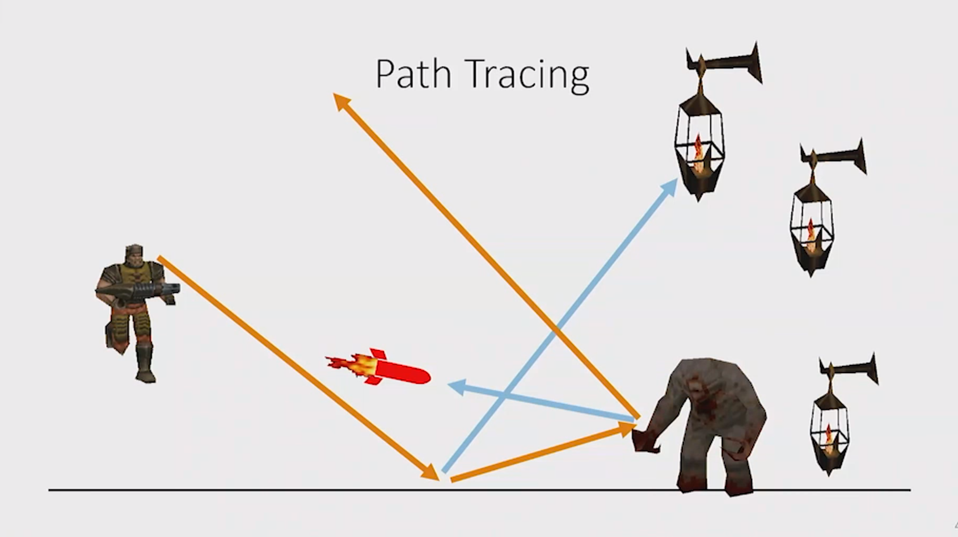
• Path tracing is a physically-based method for constructing light paths. It works by starting from the eye of the observer and casting a ray to find the primary visible surface.
• A next-event estimation is performed at the hit point. One of the light sources is stochastically selected. This can be a physically-based light source.
• All candidates are taken, and a stochastic sampling taken. Ultimately, one candidate computes the shadow ray.
• Next, we compute a scattering event. The BRDF is sampled yielding a random direction for the scattering ray.
• The next event estimation is performed for the indirectly visible surface by finding all the suitable light sources, selecting one randomly. The shadow ray is then computed.
• This process goes continues recursively.

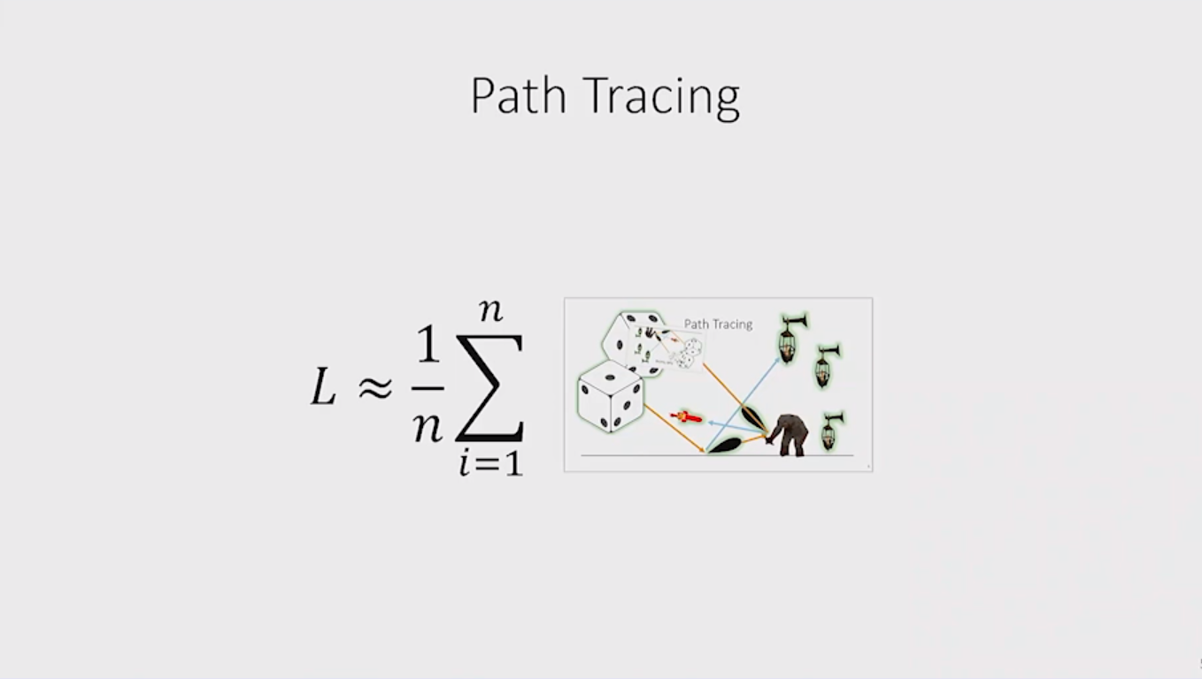
• This is a stochastic process, using random light paths. A perfect result would require infinite samples, which will never be affordable. Current technology only permits very low sample counts.
• Q2VKPT uses only one sample per pixel (i.e. one of these stochastic light paths).

• Perfect importance sampling will never be possible. This would require already solving the rendering equation, i.e. the desired result
• Full path tracing deals with much more noise than only sampling a single effect, such as indirect illumination

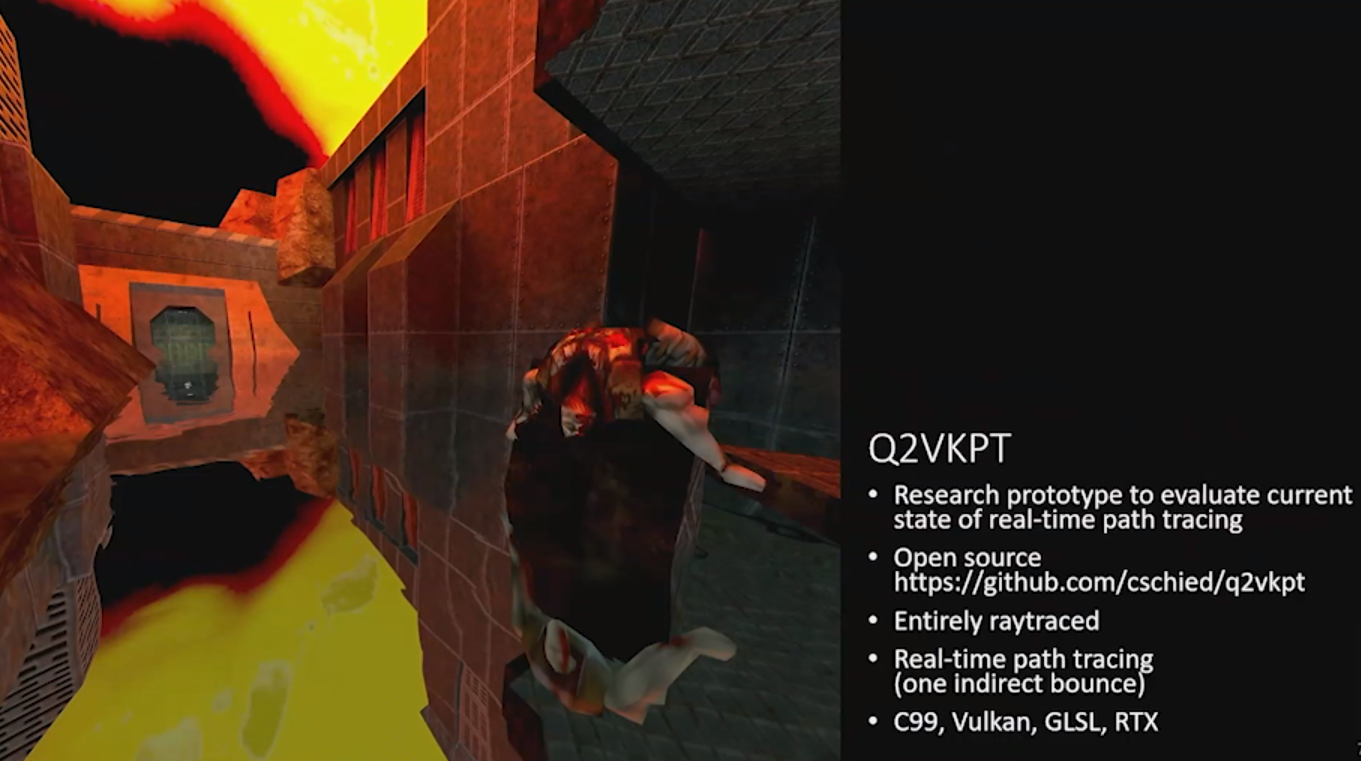
• Q2VKPT was started as a research project with the goal of figuring out the current state-of-the-art for path tracing in real time and determine if denoisers could deal with Quake 2’s fully dynamic content.
• Q2VKPT is completely open source, consisting of roughly 12,000 lines of code. It took roughly two months to write.
• It’s a completely ray traced engine, completely replacing the original renderer..
• Final result includes water reflections and explosions that work as area light sources.
• The engine computes everything fully dynamically.
• The game runs at roughly 60 fps.
• The path tracer makes up the main part of the runtime with the denoiser the second most demanding component.
• A full denoiser for path tracing is possible in 3.5 milliseconds at 1440p.

Part 2: Denoising (10 Minutes 18 Seconds)

Key Points to Remember:

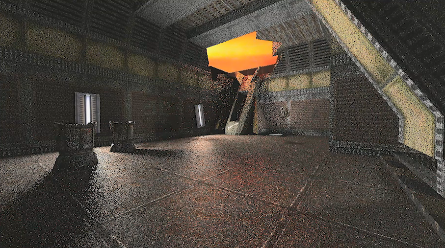
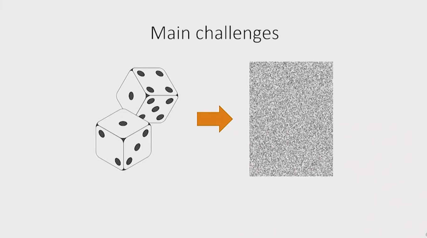
• Path tracing sees the image above as an input. It’s the raw output of the path tracer, and is very noisy.

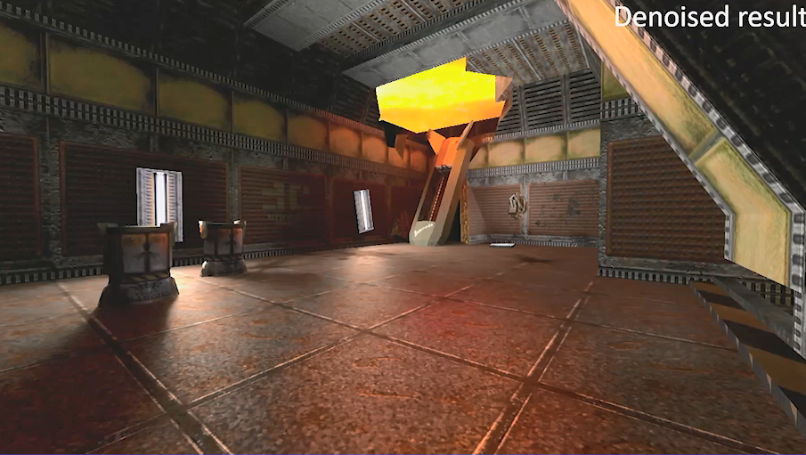
• The denoiser wipes away the noise and provides a clean image.

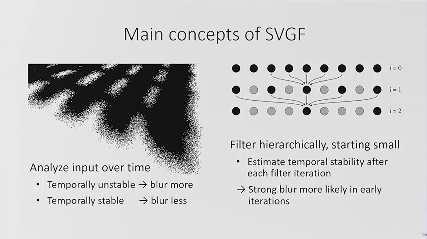
• SVGF Stands for “Spatiotemporal Variance-Guided Filtering”
• SVGF has two main principles. First, it looks at the denoising input that you pass to the denoising filter over time. Second, it stops applying blur after temporal stability is achieved.
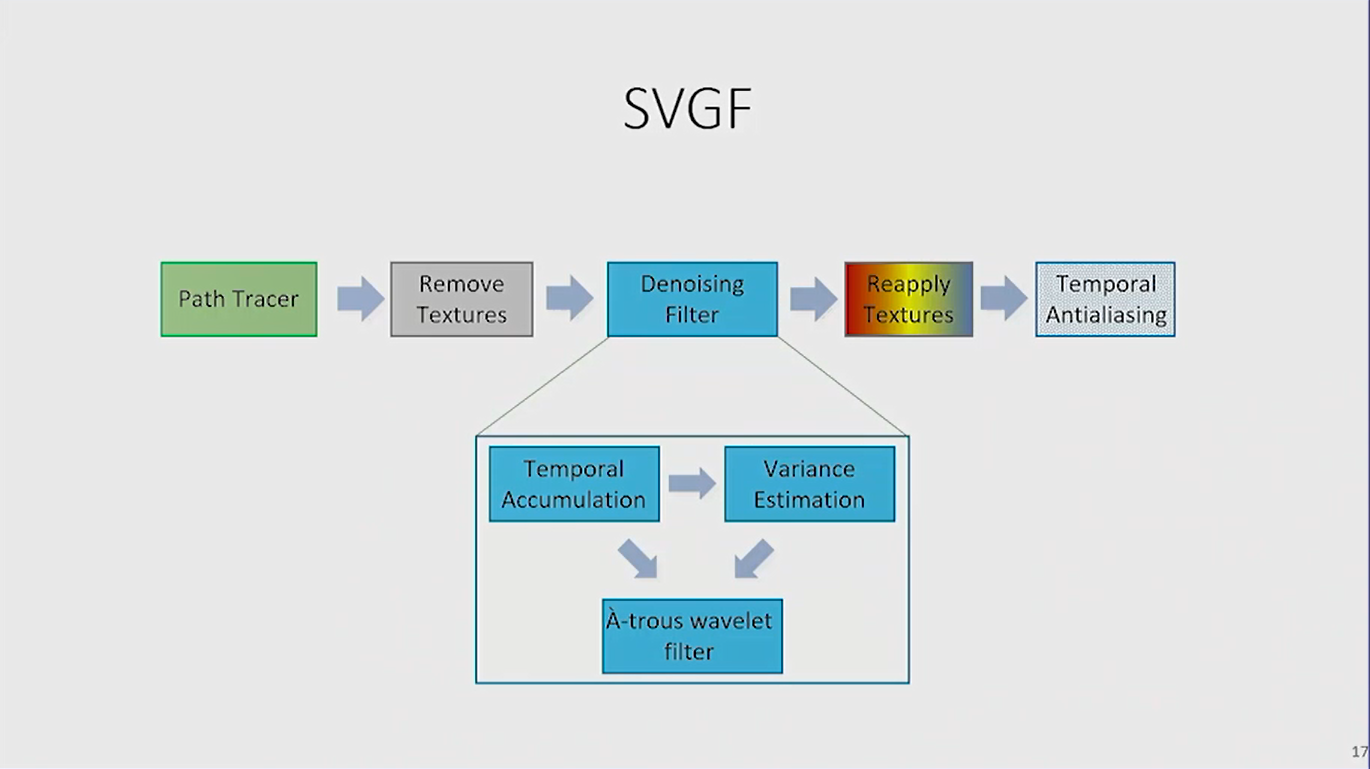
• The path tracer outputs noisy pictures. We correct for this first by removing the texture detail from the first visible surface, leaving untextured illumination. This is much easier to handle, because we do not have to protect the texture detail from the denoiser, alloign aggressive filtering. Then we remove the noise, re-apply the textures, and use TAA for some edge anti-aliasing.
• The filter itself consists of three parts, temporal accumulation, variance estimation, and A-trous wavelet filter.
• Temporal accumulation is a filter that increases the effective sample count by collecting data over time. This filter also keeps track of the noise, to steer the other parts.
• Variance estimation analyzes the image: how noisy it is, how strong the filter should be. It also acts as a fallback if there’s no temporal information yet.
• A-trous wavelet filter performs the spatial filtering

• The A-trous wavelet filter needs an input signal and detremins a weighted sum of your neighboring pixels.
• The weights consist of the filter kernel h. There also has to be edge-stopping functions, based on geometry, so you don’t blur over depth discontinuities or end up with different surface orientations.
• The most important weight is determined by comparing the difference of the luminance of the central pixel and the neighboring pixels that are combined. It is what does the heavy lifting for protecting the details.  

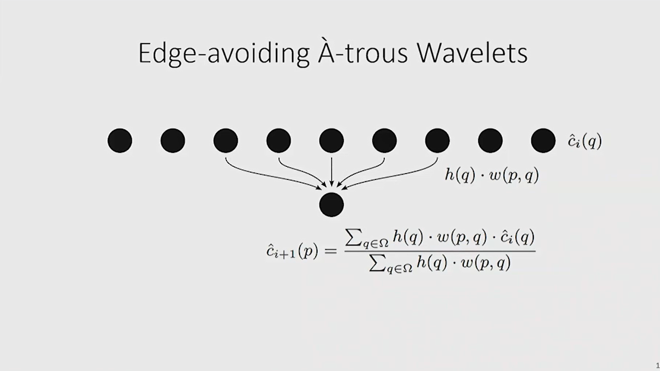
• The filter kernel is spread out. The same number of tabs exist but the effective footprint can be increased by spreading out the filter kernel. This is called strided convolution in the deep learning community.
• Each of the pixels in the previous generation already contains information from a neighborhood. This means that it’s growing very rapidly, so you need very few iterations.
• Q2VKPT only used a 3×3 box kernel and five filter iterations. That’s why the game is so efficient.
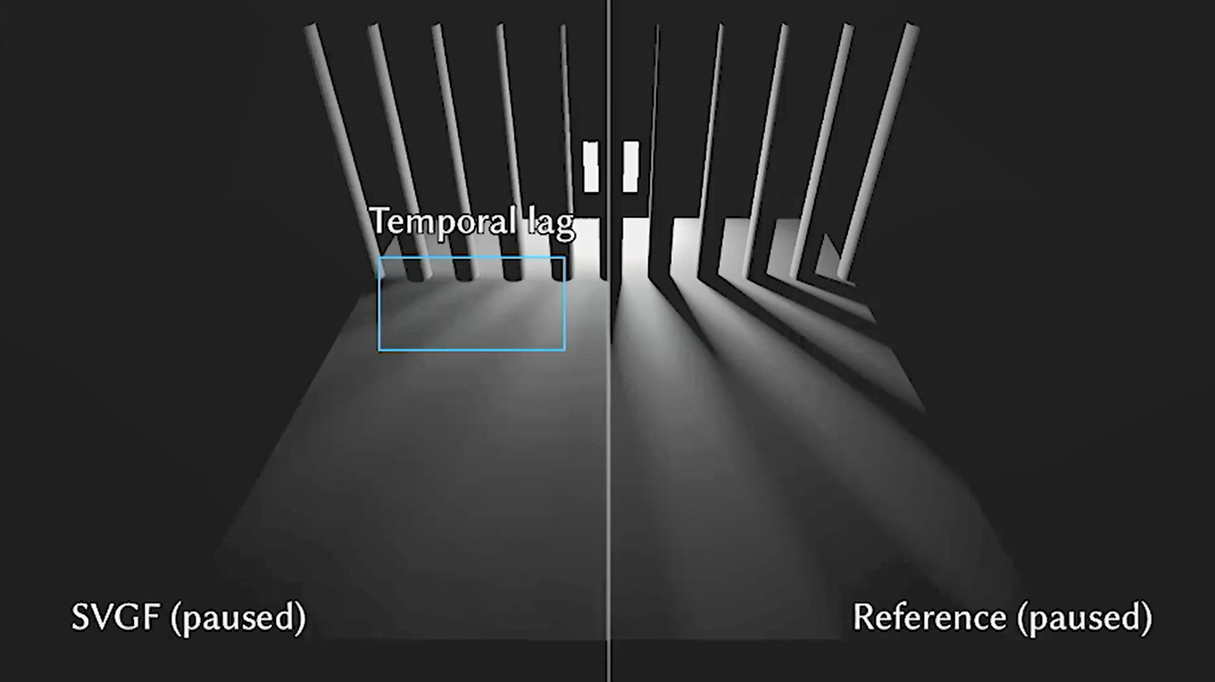
• SVGF comes with some challenges. If you look at an animated scene where there are moving occluders in front of a light source, shadows will lag behind, and won’t be fully saturated since SVGF uses a very simple temporal filter.

• Temporal filtering is very hard for path-tracing.
• The solution: adaptive temporal filtering. This replaces the simple temporal accumulation.  
• This adaptive temporal filter is also a screen space reprojection technique. The current frame, the previous frame, and motion vectors make clear (in a backwards direction) where your pixel from the current frame existed in the previous frame.

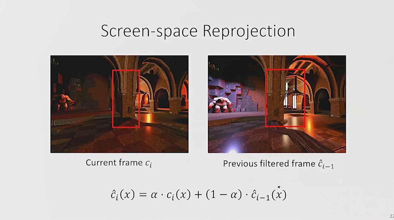
• The figure above shows a simple formula to weight the old image compared to the new image.
• If using animated camera, Geometric disocclusions may result if using an animated camera.
• You could see windows in the example from Q2VKPT (above) before they were occluded. On the right, the history for those pixels were no longer valid. Solve this required using geometric tests to verify whether we saw the same surface.
• Situations also arose where a changing of the shading function happened. Note the white reflection on the floor as an example in the image above. They are hard to detect, given the high level of noise. These shading functions are handled in a temporal filter.
• When we have an exponentially moving average, we adaptively set an alpha perimeter to be able to reliably drop history information when we detect it’s not valid anymore. Flickering lights would be a good example.

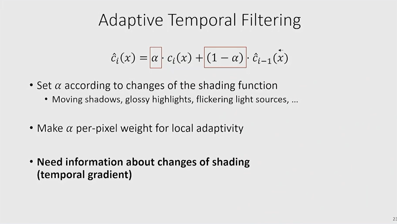
• We recommend making things locally adaptive, so if there are is a mix of stable and unstable regions in an image, then only the changed parts are dropped.
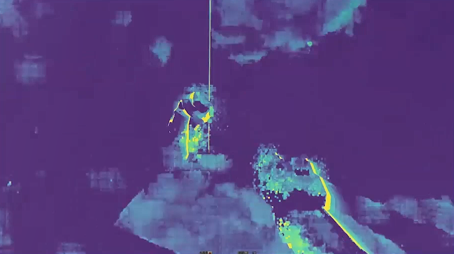
• When using an adaptive temporal filter weight, simply taking the difference between consecutive frames (above), yields very high levels of noise.
• Even using a static configuration result in high levels of noise. This makes the temporal filter completely unreliable. This level of noise will be even higher than in the original path tracer had!
• Instead of denoising, we correlated the random numbers. For each pixel we always had the same random number seed. This ensures a stable pattern of noise. If the per-pixel differences are observed, distinctive regions will be clear.
• Unfortunately, this process alone did not yield useful information. We got no new information because everything was correlated! Each frame was computing the same thing.
• For that reason, we only correlated a small subset of the pixels in the temporal filter (every ninth pixel at most).

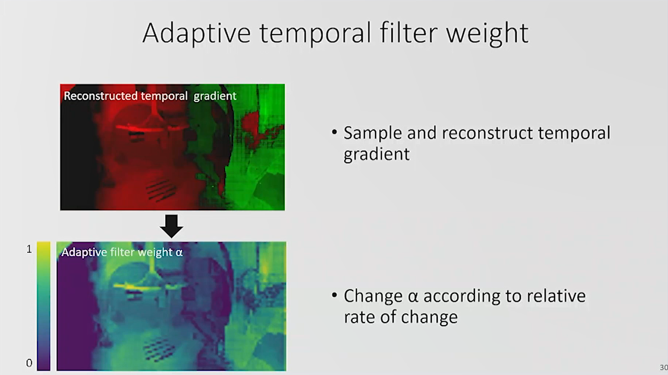
• We ended up with a very noisy and sparse temporal gradient. In this case, using a reconstruction filter (similar to SVGF) yields a dense and relatively smooth image.
• Some artifacts and noise can still be seen in the top image above.
• We wanted to understand the rate of change.
• We included additional normalization factor which told us how much the image in this region actually had changed.
• This controlled the Alpha Perimeter.

• Yellow indicates that the history has been completely dropped in the image above. All the geometric disocclusions can be seen, as well as explosions that light up the pathways.
• Also note the glossy highlights on the floor.
• These highlights show up in these gradients, and this is where the filter will drop the history.
• If you don’t do this, you will have horrible ghosting artifacts.

Part 3: Path Tracer (8 Minutes)

Key Points to Remember:

• The scene above was illuminated by A fairly large number of light sources illuminated the scene shown above. Each light source consists of several triangles.
• We turned these into an area light source. Explosions contributed to this, as well.
• If these lights had been randomly sampled from these lights, very high amounts of noise would result.
• Another challenge is that Q2VKPT doesn’t have “rooms”, it has open levels. It has to deal with full levels and therefore needs some ways to (conservatively) cull away light sources.

• Using a light hierarchy model was the first attempt at solving for the complex lighting challenges in Q2VKPT (a standard process in offline rendering).
• This model consists of a tree of light sources with stochastic traversal performed using random numbers through the light hierarchy.  
• This ended up being a nightmare for the GPU because you are maximizing how divergent your axes to the memory are.
• The quality looked inconsistent. For instance, if a  rocket flew through the scene, the topology of the tree completely changed, so everything would flicker.
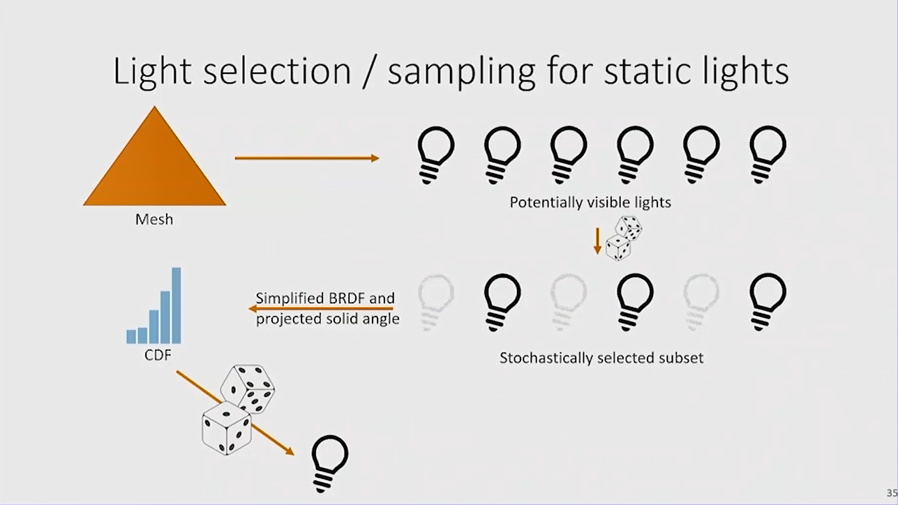
• The team ultimately went for a simpler solution, using the potentially visible set from Q2VKPT.
• This made clear on a cluster of the map which light sources would actually be visible. This was encoded as a list to be part of the mesh on the GPU.
• We then stochastically sampled from this light list. This can still be roughly 20 candidates, so we randomly select a subset and perform an expensive important sampling on top of that.
• We have a simplified version of the BRDF and also considered the projected solid angle of these triangles, building a CDF from that. We had a point-specific CDF, so the sampling quality is quite good.
• After sampling the CDF, we had one candidate for the light sources.
• This is what we do for the static lights that are part of these levels.

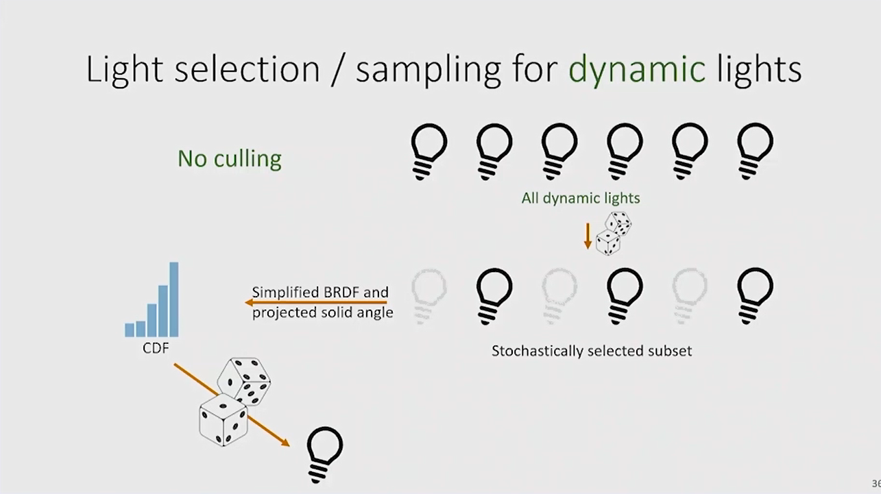
• Unfortunately, the visibility information is not pre-computed for dynamic lights.
• Given this, we didn’t do any culling, since it’s expected that the rockets are always somewhat close to the player, not somewhere else on the map.

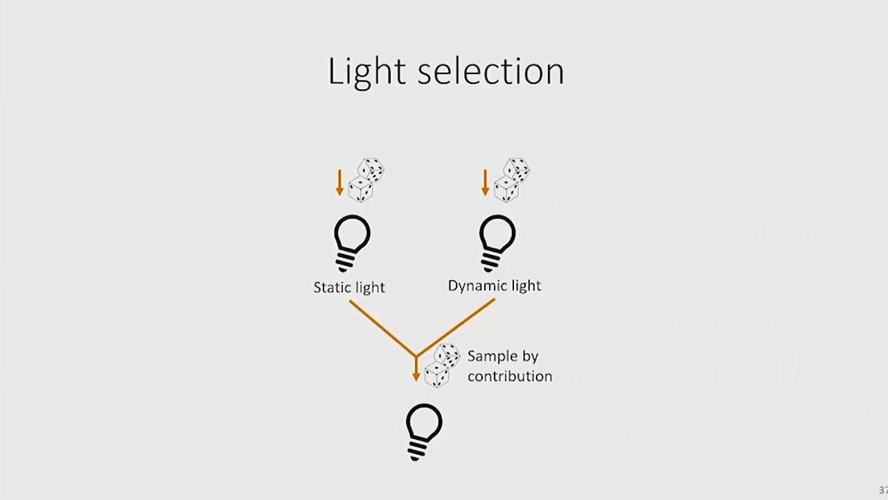
• Then, we selected between static and dynamic light sources. We could only afford one of the shadow rays. So we stochastically selected whether we wanted to sample the visibility for the static or dynamic light. We ended up with one light source in the end.

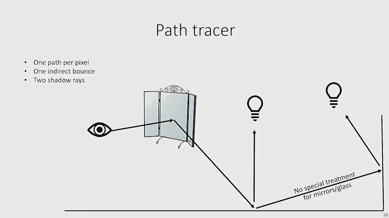
• The path tracer can handle one indirect bounce. It was still missing one ray so it could not hit the environment map from the indirect bounce.
• We had to perform two next-event estimations.
• We then had to perform two shadow rays.
• We shot the scattering ray to find the indirectly visible surface.
• We could handle glass and mirror reflections, but there were some challenges with the reconstruction filter, so we just ignored these materials for the indirect bounce.

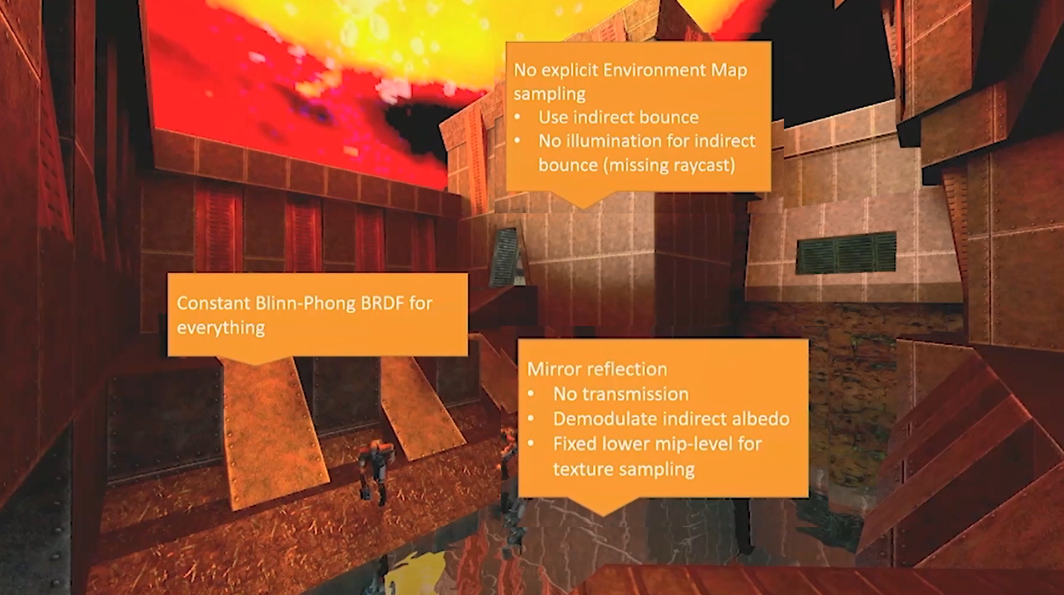
• Everything is rather metallic-looking in the screenshot above because it’s using a constant Blinn-Phone BRDF (even if it’s grass, or enemies). We didn’t pursue this further due to time limitations.
• We had direct illumination by the sky.
• The scenes included mirror reflection for water, but we did not sample the fresnel term, so it looks a bit metallic.

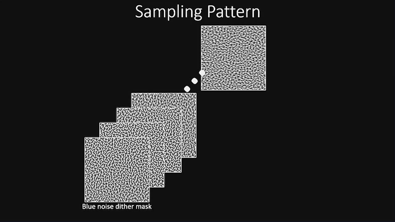
• We used a blue noise dither mask for a sampling pattern.
• For each random decision that we needed to take, we had yet another blue noise dither mask.
• We used multiples of these for the individual frames, which we recycled through. Since we needed to fill the whole screen with noise, we just tiled the blue noise dither masks.

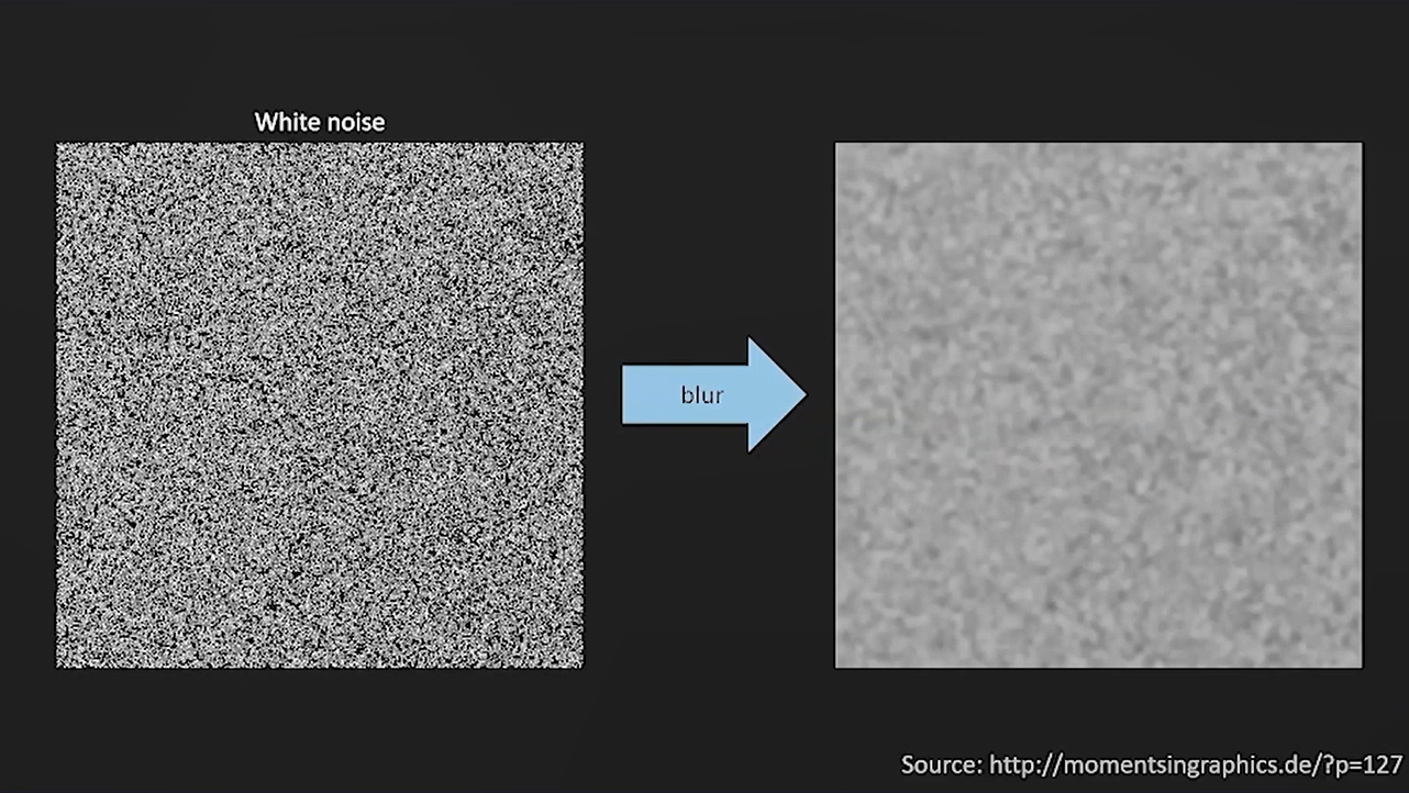
• If you use White noise with a low pass filter, lots of noise is still left in the result (see image above). This would be unstable if you look at this over time.

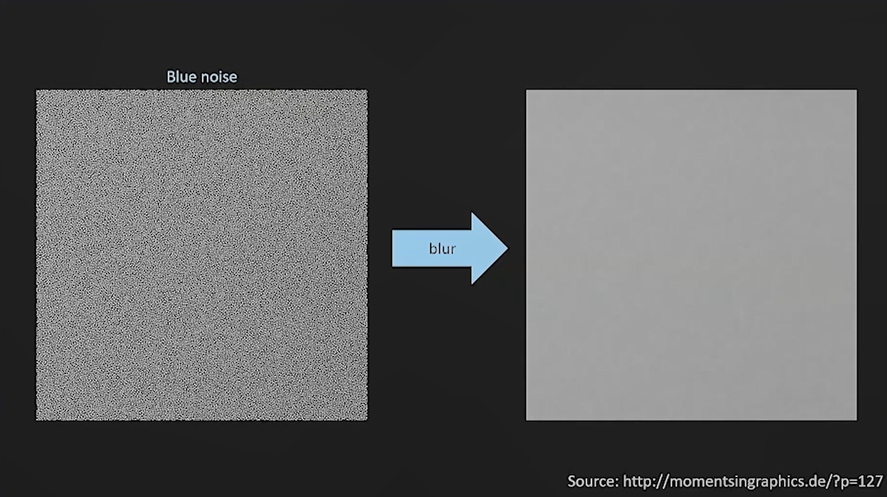
• If we do the same with blue noise, we get a much more uniform color, resulting in far less noise.  

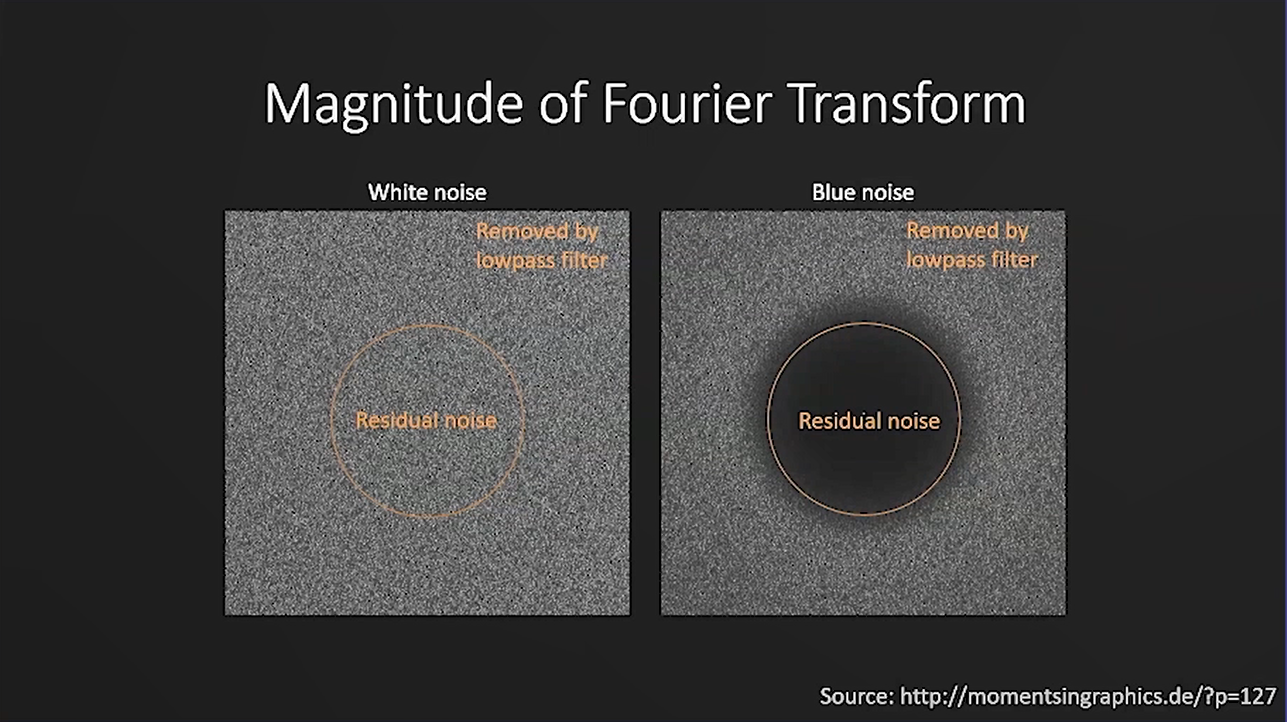
• If we look at the frequency spectra of the noise, then it is very obvious why this is happening. White noise has a full spectrum of frequencies, while blue noise has the low frequencies removed.
• We use a simple low-pass filter to denoise to make sure we did not over-blur details. You cannot remove all of the noise with the low-pass filter if you’re already starting with white noise.

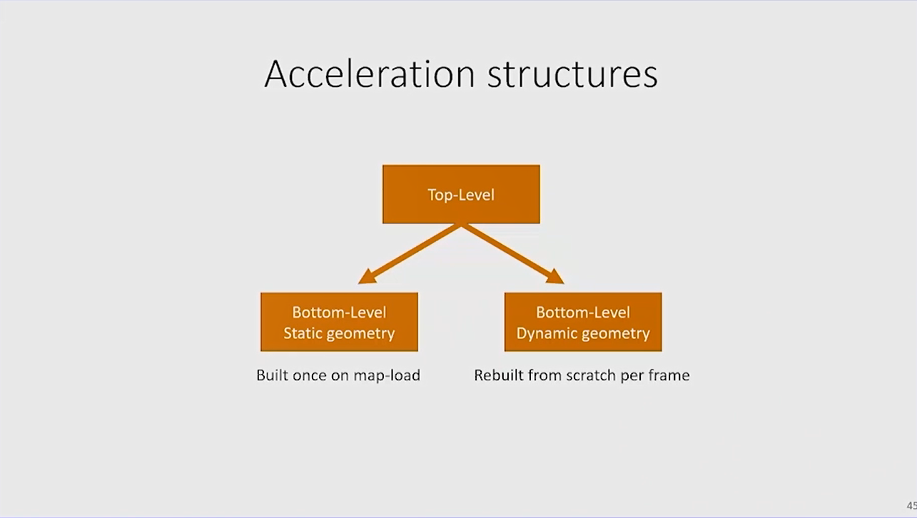
• We had two acceleration structures.
• Bottom level static geometry was built once on map-load.
• Bottom level dynamic geometry was rebuilt from scratch per frame. There were so few polygons that individually updating the parts wasn’t worth it.

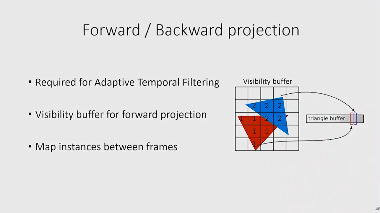
• We needed to perform a forward projection for the temporal filter for these gradient samples because we had to be very precise. This was more involved to implement, so we used a visibility buffer.
• Per pixel, we stored which of the triangles were hit. We needed to be able to map from previous to current frame.

Final Thoughts

Real-time path tracing is possible (in the near future), but the transition can be difficult. You need random access to everything as well as having to tweak the assets. More research specifically tailored towards real-time rendering needs to take place, including digging into fast and robust importance sampling and denoising.

The entire talk can be viewed on the NVIDIA Developer website (you must be an NVIDIA Registered Developer to view), which includes an additional 25 minute breakdown of the making of Quake II RTX from an NVIDIA engineer’s perspective.

If you are working on ray-traced games, we also recommend looking at our newly released Nsight Graphics 2019.3, a debugging and GPU profiling tool which has been updated to include support for DXR and NVIDIA VKRay.