Optimizing LLMs for Performance and Accuracy with Post-Training Quantization

Quantization is a core tool for developers aiming to improve inference performance with minimal overhead. It delivers significant gains in latency, throughput, and memory efficiency by reducing model precision in a controlled way—without requiring retraining.

Today, most models are trained in FP16 or BF16, with some, like DeepSeek-R1, natively using FP8. Further quantizing to formats like FP4 unlocks substantial efficiency gains and performance, supported by a growing ecosystem of open-source techniques.

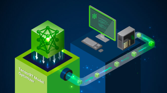
NVIDIA TensorRT Model Optimizer post-training quantization (PTQ) framework offers a flexible and modular approach to applying these optimizations. It supports a broad range of formats, including NVFP4, optimized for NVIDIA Blackwell GPUs, and integrates calibration techniques like SmoothQuant, activation-aware weight quantization (AWQ), and AutoQuantize for improved quantization results.

Model Optimizer PTQ is also ecosystem-friendly, supporting native PyTorch, Hugging Face, NeMo, and Megatron-LM checkpoints while easily integrating with inference frameworks such as NVIDIA TensorRT-LLM, vLLM, and SGLang.

This post expands on PTQ techniques and introduces how to use Model Optimizer PTQ for compressing AI models while maintaining high accuracy, which enhances the user experience and AI application performance.

Introduction to quantization

Neural networks are composed of layers containing values that can be tuned through model pre- and post-training processes and learn to perform different tasks. These learnings are stored as weights, activations, and biases across different types of layers. In practice, models are typically trained at full precision (TF32/FP32), half-precision (BF16/FP16), mixed precisions, and, more recently, FP8. The training precision determines the native precision of the models, which directly contributes to both the computational complexity and memory requirements of performing inference with that model.

Quantization enables us to trade excess precision typically needed during training for faster inference and a smaller memory footprint. Performance gains depend on how much of the network we quantize, the difference between native and quantized precision, and the algorithm we use. Figure 1 shows how a group of high-precision weights can be resampled and quantized.

Illustration of the quantization process: The top row shows evenly spaced original weights at baseline precision. An arrow points to a lower section where these weights are mapped onto a bell‑curve‑like distribution, aligning each original value to the nearest available level in a lower‑precision quantized format, represented by discrete boxes. — *Figure 1. A simple illustration of how quantization is essentially a resampling of values from high to lower precision formats*

32-bit and 16-bit data types, typically used in model training, can be quantized down to 8-bit, 4-bit, and beyond. This process involves compressing the original values to fit the smaller representable ranges of lower precision data types.

During this quantization process, values must be adapted to the representable range of the target data type. During this adaptation, the values range from more to less granular. For example, going from FP16 to FP8, the values A and B, after quantization, are represented as QA and QB, but further apart, resulting in lower resolution (Figure 2).

Comparison of representable ranges and data precision for FP16, FP8, and FP4 formats. — *Figure 2. What happens to range and detail when we quantize from FP16 down to FP*8 or FP4

The representable ranges for the most popular data types are summarized in Table 1 below.

Data Type	Total Bits	Representable Range
FP32	32	±3.4 × 10³⁸
FP16	16	±65,504
BF16	16	±3.4 × 10³⁸
FP8	8	±448
FP4	4	-6 to +6
INT8	8	-128 to +127
INT4	4	-8 to +7

Table 1. Summary of data types with bit width, representable ranges, and format descriptions (floating point vs. integer)

The resulting quantization format will have a version of the original values represented in the quantized format’s range. This conversion is achieved using a quantization scaling factor, which is calculated using the following formula.

$\boldsymbol{S} = \frac{\boldsymbol{2}^{\boldsymbol{b} - \boldsymbol{1}} - \boldsymbol{1}}{\boldsymbol{\alpha}}$

Where b is the target byte count, and $\alpha$ is the highest absolute value present in the original data type. The quantized value is calculated using the following formula.

$\boldsymbol{X}_{\text{quantized}} = \mathit{round}(\boldsymbol{S} \cdot \boldsymbol{X})$

Where X is the original data type, and S is the scale factor. Figure 3 shows the results of the quantization process converting from FP16 to FP4. The FP16 values {4.75, 2.01, -3.44, -7.11, 0, 13.43, -4.91, -6.43} are quantized to {2, 1, -2, -4, 0, 7, -3, -3} in FP4.

Illustration of symmetric static quantization. The mapping shows how higher‑precision floating‑point values are compressed into lower‑precision representations while preserving relative relationships. — *Figure 3. Example of scaling FP16 values down to FP4 using symmetric static quantization and standard scaling factors*

There are many techniques for adapting quantization, but this blog post focuses on effective PTQ using Model Optimizer. While there are many advanced methods like clipping, range mapping, and calibration, Model Optimizer provides a simple API to make it easy to apply the right configuration.

PTQ with TensorRT Model Optimizer

TensorRT Model Optimizer is a library of advanced model optimization techniques dedicated for optimizing the inference performance of models. After the models have been optimized, they can be deployed downstream using inference frameworks like Dynamo, SGLang, TensorRT-LLM, and vLLM.

Table 2 provides a summary of the different quantization formats supported by Model Optimizer and a brief description.

QuantizationFormat	Description
Per-Tensor FP8	Standard full-model FP8 quantization using default scale encoding
FP8 Block-wise Weight Only	2D block-wise, weight-only quantization. Shared scaling across small blocks.
FP8 Per Channel and Per Token	Per-channel weights, dynamic per-token activations quantization.
nvfp4	Default FP4 quantization for weights and activations.
INT8 SmoothQuant	8-bit quantization with SmoothQuant calibration. Per-channel weights, per-tensor activations.
WA416 (INT4 Weights Only)	4-bit weight-only quantization with AWQ calibration. Group-wise/block-wise weights, FP16 activations.
W4A8 (INT4 Weights, FP8 Activations)	4-bit weight, FP8 activation quantization with AWQ. Block-wise weights, per-tensor FP8 activations.
fp8 (KV)	Enables FP8 quantization of key-value caches in attention layers
nvfp4 (KV)	FP4 cache quantization for key-value caches in transformer attention layers.
Nvfp4_affine (KV)	Key-value cache quantization using affine scaling.

Table 2. Table summarizing quantization formats supported by Model Optimizer, organized by type (floating point, integer, KV cache), with descriptions

Choosing the right quantization format, KV cache precision, and calibration method depends on your specific model and workload. Model Optimizer offers several techniques to help with this, including:

Min-max calibration
SmoothQuant
Activation-aware weight quantization (AWQ)
AutoQuantize

In the following sections, we’ll walk through these techniques in detail and provide hands-on Jupyter notebook tutorials so you can learn how to use the Model Optimizer API and apply it to your own models.

Standard quantization with min-max calibration

Before a model can be quantized, it needs to be calibrated to understand the dynamic range of its activations. One of the simplest and most common calibration methods is min-max calibration. In this process, a small, representative dataset (calibration dataset) is passed through the original model to collect activation statistics. For each tensor, the minimum and maximum values observed are used to determine the scaling factors for mapping float values to lower-precision integers. While fast and easy to apply, min-max calibration can be sensitive to outliers and lacks the adaptive scaling used in more advanced techniques

Assuming the model and tokenizer have been successfully loaded, the calibration data loader and forward loop can be configured using the get_dataset_dataloader and create_forward_loop utility functions provided by Model Optimizer. PTQ can be applied using a small calibration dataset—typically just 128 to 512 samples, and accuracy is generally stable across different datasets. In this example, the dataset cnn_dailymail is used. A different dataset can be substituted by modifying the dataset_name configuration in the get_dataset_dataloader() call.

# Calibration dataloader
calib_loader = get_dataset_dataloader(
    dataset_name=”cnn_dailymail”,
    tokenizer=tokenizer,
    batch_size=batch_size,
    num_samples=calib_samples,
    device="cuda"
)

forward_loop = create_forward_loop(dataloader=calib_loader)

Configuring the quantization parameters requires three key inputs:

The original mode
The quantization configuration
The forward loop.

In this example, we use the default NVFP4 configuration for weights and activations by setting quant_cfg = mtq.NVFP4_DEFAULT_CFG, and then apply it to the model using the mtq.quantize() function.

# Quantize with NVFP4 config
quant_cfg = mtq.NVFP4_DEFAULT_CFG
model = mtq.quantize(model, quant_cfg, forward_loop=forward_loop)

Once the quantization has been applied successfully, the model can be exported using the instructions found in the Exporting a PTQ Optimized Model section of this post. To dive deeper into this PTQ method, we recommend exploring the complete Jupyter notebook walkthrough.

Advanced calibration techniques

Calibration determines the optimal scaling factors by analyzing representative input data. Simple approaches like max calibration use the maximum absolute value in the tensor, which may lead to underutilized dynamic range. More advanced techniques like SmoothQuant balance activation smoothness with weight scaling, while AWQ adjusts weight groups post-training to maintain output distribution. The calibration method significantly impacts the final accuracy of the quantized model and should align with the workload’s sensitivity and latency requirements.

Calibration techniques can be applied to both floating-point and integer formats. In practice, they are often required for integer data types like INT8 and INT4 to recover acceptable accuracy post-quantization.

Activation-aware weight quantization

Introduced in 2023, AWQ focuses on weight quantization by considering activation ranges. The idea is to choose per-channel weight scales that minimize ‌ worst-case quantization errors given typical activation patterns.

AWQ “forgives” some weight error in channels that contribute less to outputs—due to small activations. One of AWQ’s strengths is that it enables very low-bit weight quantization (4-bit) with minimal impact by not treating all weights equally.

Diagram of the AWQ process, which prioritizes high-activation channels by applying larger scaling factors, preserving their impact in the final quantized representation. — Figure 4. *Adapted from the AWQ paper—selective scaling of salient (high-activation) weights to preserve accuracy during quantization*

The core premise of AWQ is that it prioritizes salient weights—those deemed most active, typically due to their alignment with high-magnitude activations—and handles them with greater care during quantization. These critical weights are either quantized with higher precision or preserved in their native format, while less important weights are more aggressively quantized.

This selective approach reduces quantization error where it matters most, enabling effective use of lower-bit formats. As shown in Figure 4, each channel is selected based on average magnitude and carefully scaled prior to quantization, helping preserve the influence of the most impactful weights.

The Model Optimizer API enables users to override parameters such as block size for fine-grained control over the quantization process. For a complete walkthrough, reference the min-max quantization Jupyter notebook.

SmoothQuant

Introduced in 2022, SmoothQuant addresses the issue of activation outliers resulting from low-precision quantization. In transformer architectures, layers can have highly skewed activation distributions (e.g., very large values in certain channels due to the scale of attention computations for Q/K/V), which makes straightforward quantization risky.

Figure 5 shows the basic intuition of the SmoothQuant process. Starting with an original distribution of activations and corresponding outliers |X|. These values are scaled down to create $\boldsymbol{|\hat{X}|}$ , and |W| is scaled up accordingly to create $\boldsymbol{|\hat{W}|}$ so that the product remains mathematically valid.

Model Optimizer AutoQuantize

The Model Optimizer AutoQuantize function is a per-layer quantization algorithm that uses a gradient-based sensitivity score to rank each layer’s tolerance to quantization. This enables it to search for and select the optimal quantization format—or even skip quantization—on a layer-by-layer basis (Figure 6).

The process is guided by user-defined constraints, such as the effective_bits parameter, which balances higher throughput needs with the preservation of model accuracy. By tailoring quantization at the layer level, the algorithm can aggressively compress less sensitive layers while preserving precision where it matters most. Users can also apply varying levels of compression based on specific hardware targets and model requirements, offering fine-grained control to optimize deployment efficiency across diverse environments.

An AutoQuantize diagram. On the left, two sample quantization formats (INT8 and NVFP4) are shown. On the right, icons for capturing measured accuracy and performance metrics, illustrating how AutoQuantize evaluates different formats layer by layer to find the optimal balance between accuracy and efficiency. — *Figure 6. Simplified animation of the AutoQuantize workflow—evaluating and selecting optimal per-layer quantization formats (e.g., INT8, NVFP4) based on accuracy and performance trade-offs*

The resulting model will use a customized quantization scheme, applied according to the candidate configurations provided to the auto-quantization function. When the search space per layer is large, this technique can result in higher computational costs and longer processing times compared to the other methods discussed in this post. To reduce complexity, you can choose a smaller set of candidate configurations and skip KV cache calibration.

Applying AutoQuantize using the Model Optimizer API is quite straightforward. It starts with identifying the pool of quantization configuration for weights and the KV quantization config for activations. The accompanying Jupyter notebook dives deeper into different configurations and how to apply them effectively.

Results of quantizing to NVFP4

The previous sections provided an overview and initial introduction to the implementation of various PTQ techniques. The effectiveness of each technique, in terms of the resulting inference performance boost and model accuracy, varies depending on the exact recipe and hyperparameters used.

NVFP4 provides the highest level of compression offered by Model Optimizer PTQ, providing stable accuracy recovery and significant increases in model throughput. Figure 8 below cross-plots the impact on accuracy and output token throughput after quantization from their original precision to NVFP4. NVFP4 quantization dramatically increases token generation throughput for major language models—such as Qwen 23B, DeepSeek-R1-0528, and Llama Nemo Ultra—while maintaining nearly all of their original accuracy, as shown by high relative accuracy percentages even at 2-3x speedup.

This scatter plot shows the relationship between throughput speedup and accuracy retention for large language models quantized with NVFP4. The chart visually demonstrates that NVFP4 quantization delivers substantial inference speedup with minimal loss in model accuracy. — *Figure 8. Cross-plot showing NVFP4 token generation throughput speedup and accuracy impact*

The following chat demo showcases the equal fidelity of a response to a Deepseek-R1 query, but the much faster response from the NVFP4 quantized model compared to the FP8 baseline.

Side‑by‑side comparison of DeepSeek‑R1 chat responses at different precisions, demonstrating that NVFP4 maintains response fidelity while enabling faster inference performance. — *Figure 9. Chat demo comparing DeepSeek‑R1 responses—showing equal fidelity but faster output with NVFP4 quantization vs. FP8*

This combination of performance boost and accuracy retention enables efficient TCO optimization with virtually no change to the fidelity of the AI workload.

Exporting a PTQ optimized model

Once you have selected and successfully applied the desired PTQ technique, the model can be exported to a quantized Hugging Face checkpoint. This is similar to the common Hugging Face checkpoints, which makes it easy to share, load, and run models across various inference engines like vLLM, SGLang, TensorRT-LLM, and Dynamo.

Exporting to a Quantized Hugging Face checkpoint

from modelopt.torch.export import export_hf_checkpoint

export_hf_checkpoint(model, export_dir=export_path)

Want to try PTQ-optimized models right away? Check out the pre-quantized model checkpoints on the Hugging Face Hub. The NVIDIA Model Optimizer collection includes ready-to-use checkpoints for Llama 3, Llama 4, and DeepSeek.

Summary

Quantization is one of the most effective ways to supercharge model inference—delivering big wins in latency, throughput, and memory efficiency without the cost of retraining. While most large models today run in FP16 or BF16 (and some, like DeepSeek‑R1, in FP8), pushing even further to formats like FP4 unlocks a whole new level of efficiency. Backed by a rapidly growing ecosystem of techniques, this shift is transforming how developers deploy and scale high‑performance AI.

NVIDIA TensorRT Model Optimizer takes this to the next level. With support for cutting‑edge formats like NVFP4 (built for NVIDIA Blackwell GPUs), advanced calibration strategies such as SmoothQuant, AWQ, and AutoQuantize, and seamless integration with PyTorch, Hugging Face, NeMo, Megatron-LM, vLLM, SGLang, TensorRT‑LLM, and Dynamo, giving developers a powerful toolkit for compression without compromise. The result? Faster, leaner, and more scalable AI deployments that preserve accuracy and elevate the user experience. If you’re ready to see these benefits in action, explore our Jupyter notebook tutorials or try the pre‑quantized checkpoints today.