WaveNets represent an exciting new neural network architecture used to generate raw audio waveforms, including the ability to synthesize very high quality speech. These networks have proven challenging to deploy on CPUs, as generating speech in real-time or better requires substantial computation in tight timeframes. Fortunately, GPUs offer the tremendous parallel compute capability needed to make high-throughput, real-time WaveNet deployment a reality using nv-wavenet.
In this post, I’ll introduce nv-wavenet, a reference implementation of a CUDA-enabled autoregressive WaveNet inference engine. More specifically, the implementation targets the autoregressive portion of the WaveNet variant described by Deep Voice. It includes several different implementation variants, allowing tradeoffs between complexity, maximum sample rate, and throughput at a given sample rate.
Several groups have recently put forward alternatives to autoregressive WaveNet such as Parallel WaveNet and WaveRNN. While these alternatives also work well on GPUs, I will focus exclusively on autoregressive WaveNet inference. Our research has shown that autoregressive WaveNets provide high quality results yet are simple to train. Accordingly, fast inference kernels for autoregressive WaveNets are valuable for both deployment directly as well as for increasing researcher iteration speed during the training of text-to-speech models.
Autoregressive WaveNet Inference
Autoregressive WaveNets can be challenging to deploy, since the input to each timestep of the model includes the output of the model for a prior timestep. Consequently, the deployment has a long sequential critical path. To understand why that can be a problem, let’s take a look at a dilated convolution such as that employed by WaveNets, shown in figure 1.
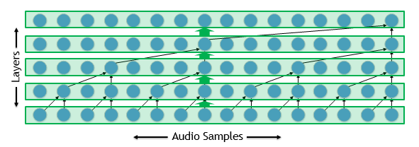
Implementing the network is straightforward for training: we implement each layer with one or more kernels. These kernels run parallel across the many thousands of audio samples in our waveform and can run quite efficiently.
On the other hand, we have to wait for the model to produce a single sample before we can begin processing the next sample for inference, as shown in figure 2.
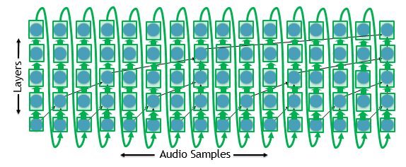
Let’s assume we want to generate a waveform at 24 kHz. We only have 42.7 microseconds to produce each sample given their sequential dependency. That gives us just over a microsecond for each layer for a 40-layer model. Running a GPU kernel in a microsecond is impractical, so let’s try something different.
Figure 3 demonstrates that one option is to launch a kernel for a single timestep rather than for a single layer.
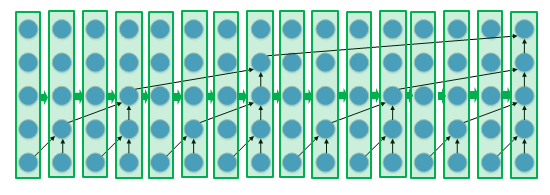
This requires a much more sophisticated kernel since it must implement the entire model. However, we now have the full 42.7 microseconds instead of a meager 1 microsecond per kernel. To take it further, if we’ve already gone to the trouble of implementing the entire model in a single kernel, we might as well use that kernel to generate multiple samples per call. This frees us from concerns about kernel overheads entirely.
Introducing nv-wavenet
nv-wavenet is an open-source implementation of several different single-kernel approaches to the WaveNet variant described by Deep Voice. The implementation focuses on the autoregressive portion of the WaveNet since it’s the most performance-critical. The conditioning data which determines what speech to produced must be provided from an external source.
Three implementation variants of nv-wavenet currently exist: single-block, dual-block, and persistent.
Single-block variant
Figure 4 shows the single-block variant, which implements the entire model in a single thread block.
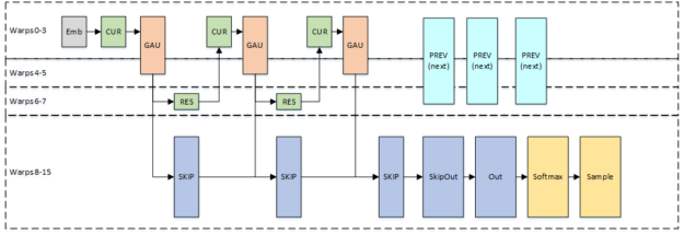
PREV and CUR are the two halves of the 2×1 dilated convolution. PREV processes data from a prior timestep, determined by the layer dilation, while CUR processes data from the current timestep. GAU, the Gated Activation Unit, comprises a tanh and sigmoid followed by a pointwise multiplication. RES and SKIP make up the final convolution in the residual layer. RES produces the residual channels and SKIP produces the skip channels. Since the PREV computations only depend on the residual layers, we overlap the PREV computations for the next sample with the final layers of the current sample in order to reduce the total sample generation time.
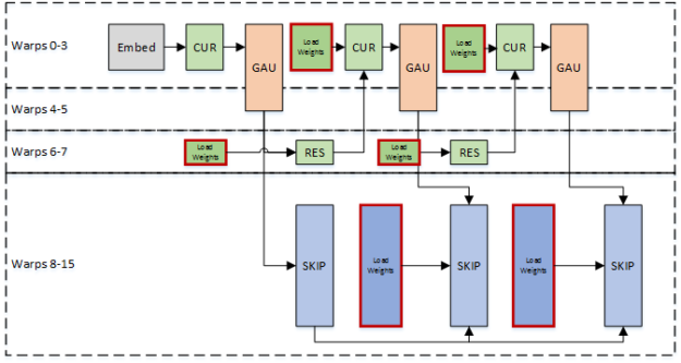
Since the thread block must load the weights for the entire model for each generated sample, our maximum sample rate is limited by the read bandwidth of a single Streaming Multiprocessor. We use warp specialization to pipeline the weight loads with computation to use the bandwidth most effectively. Some warps load weights while other warps perform the computation, as shown in figure 5.
Scaling throughput
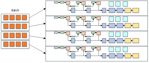
If we implement the entire model in a single block, a single inference can only use one Streaming Multiprocessor. This is an ineffective use of resources on a Tesla V100 GPU which has 80 Streaming Multiprocessors. We can simply increase the number of inferences we’d like to perform by launching multiple blocks in order to make better use of those idle resources. Figure 6 displays how throughput can increase even further by running a small batch per thread block as long as we balance the batch size per block against the time budget provided by our target sample rate.
Dual-block variant
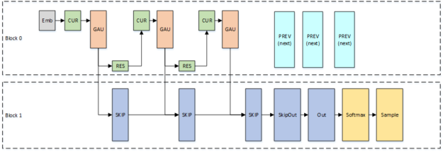
The single-block approach may not achieve our desired sample rate if the model is too large. One simple alternative: split the model across two thread blocks. Since these thread blocks can run on different Streaming Multiprocessors, we’ve effectively doubled our available bandwidth for loading model weights. Figure 8 shows how we’ve divided the model across blocks.
Persistent variant
Ultimately, we want to avoid worrying about weight bandwidth at all for very large models or very high sample rates. The persistent variant divides the model across many thread blocks, as you can see in Figure 9. Each thread block loads a subset of the weights and holds on to them for the entire waveform generation. The time-to-compute plus the inter-block communication time now limits sample rate, rather than the time to load weights.
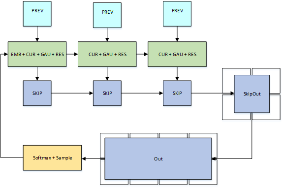
The persistent variant implements each residual layer as three thread blocks: one thread block computes the portion of the dilated convolution that computes data from a prior timestep, a second thread block implements the rest of the dilated convolution in addition to the gated activation logic and the residual convolution, and a third block implements the skip convolution. The final convolutions can be much larger and are thus implemented with multiple collaborative thread blocks.
nv-wavenet Performance
Let’s take a look at how these different variants perform on two different WaveNets described in the Deep Voice paper:
- “Medium” is the largest model for which the Deep Voice authors were able to achieve 16 kHz inference on a CPU. It uses 64 residual channels, 128 skip channels, and 20 layers.
- “Large” provides much better quality but the Deep Voice authors were unable to reach their target of 16 kHz. This model uses 64 residual channels, 256 skip channels, and 40 layers.
All data shown are for nv-wavenet compiled with CUDA 9.0 running on a Tesla V100-SXM2. While nv-wavenet supports both fp16 and fp32, we only show fp16 data.
Maximum sample rate
First, let’s look at the maximum sample rate for a single unbatched inference in Figure 10:
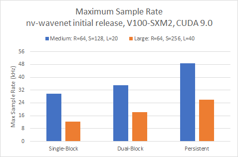
All three approaches easily exceed our real-time targets of 16 and 24 kHz for the smaller of the two models. We need to use the dual-block variant to exceed 16 kHz for the larger model while pushing higher than 24KHz requires the persistent variant.
The maximum sample rate is only part of the picture. We’d like to do many inferences in parallel to make the most of our GPU. Let’s look at the largest batch size that we can achieve while still hitting a target sample rate, shown in figure 11.
Throughput at 16 kHz
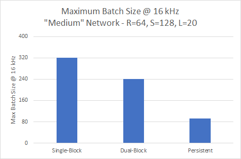
The single-block variant offers the greatest throughput efficiency of all three variants at 16KHz for the smaller model but has the lowest maximum sample rate.
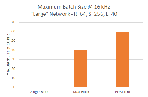
The single-block variant cannot reach 16 kHz with the larger model, so requires the persistent variant to provide the highest throughput, as you can see in figure 12.
Throughput at 24 kHz
The trend shown earlier continues for the smaller network at 24kHz. Figure 13 shows the single-block variant providing the highest throughput at a batch of 106.
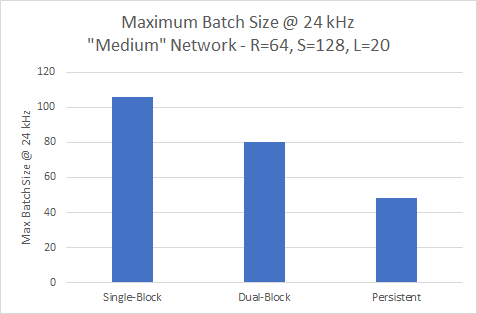
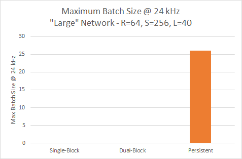
Figure 14 illustrates that only the persistent variant achieves 24 kHz for the larger model, where it can run a batch of 26.
nv-wavenet Exploits GPUs for Speech Generation
WaveNets give us an exciting approach to speech synthesis. CUDA provides an excellent platform for deploying these networks in real-time, exploiting the massively parallel compute resources of NVIDIA GPUs. I’m particularly excited NVIDIA made nv-wavenet open-source, allowing users to modify the code further to meet their unique requirements. We’ve made nv-wavenet source code available for download. If you have more questions or feedback, please take our nv-wavenet survey — it’s only a few questions and gives us better insight into your use cases. Feel free to take nv-wavenet for a spin, modify it, give us feedback on how we can make it better.


