
Analysis of statistical algorithms can generate workloads that run for hours, if not days, tying up a single computer. Many statisticians and data scientists write complex simulations and statistical analysis using the R statistical computing environment. Often these programs have a very long run time. Given the amount of time R programmers can spend waiting for results, it makes sense to take advantage of parallelism in the computation and the available hardware.
In a previous post on the Teraproc blog, I discussed the value of parallelism for long-running R models, and showed how multi-core and multi-node parallelism can reduce run times. In this blog I’ll examine another way to leverage parallelism in R, harnessing the processing cores in a general-purpose graphics processing unit (GPU) to dramatically accelerate commonly used clustering algorithms in R. The most widely used GPUs for GPU computing are the NVIDIA Tesla series. A Tesla K40 GPU has 2,880 integrated cores, 12 GB of memory with 288 GB/sec of bandwidth delivering up to 5 trillion floating point calculations per second.
The examples in this post build on the excellent work of Mr. Chi Yau available at r-tutor.com. Chi is the author of the CRAN open-source rpud package as well as rpudplus, R libraries that make is easy for developers to harness the power of GPUs without programming directly in CUDA C++. To learn more about R and parallel programming with GPUs you can download Chi’s e-book. For illustration purposes, I’ll focus on an example involving distance calculations and hierarchical clustering, but you can use the rpud package to accelerate a variety of applications.
Hierarchical Clustering in R
Cluster analysis, or clustering, is the process of grouping objects such that objects in the same cluster are more similar (by a given metric) to each other than to objects in other clusters. Cluster analysis is a problem with significant parallelism. In a post on the Teraproc blog we showed an example that involved clustering analysis using k-means. In this post we’ll look at hierarchical cluster in R with hclust, a function that makes it simple to create a dendrogram (a tree diagram as in Figure 1) based on differences between observations. This type of analysis is useful in all kinds of applications from taxonomy to cancer research to time-series analysis of financial data.

Similar to our k-means example, grouping observations in a hierarchical fashion depends on being able to quantify the differences (or distances) between observations. This means calculating the Euclidean distance between pairs of observations (think of this as the Pythagorean Theorem extended to more dimensions). Chi Yau explains this in his two posts Distance Matrix by GPU and Hierarchical Cluster Analysis, so we won’t attempt to cover all the details here.
R’s hclust function accepts a matrix of previously computed distances between observations. The dist function in R computes the difference between rows in a dataset supporting multiple methods including Euclidean distance (the default). If I have a set of M observations (rows), each with N attributes (columns), for each distance calculation I need to compute the length of a vector in N-dimensional space between the observations. There are \(M * (M-1) / 2\) discrete distance calculations between all rows. Thus, computation scales as the square of the number of observations: for 10 observations I need 45 distance calculations, for 100 observations I need 4,950, and for 100,000 observations I need 4,999,950,000 (almost 5 billion) distance calculations. As you can see, dist can get expensive for large datasets.
Deploying a GPU Environment for Our Test
Before I can start running applications, first I need access to a system with a GPU. Fortunately, for a modest price I can rent a machine with GPUs for a couple of hours. In preparing this blog I used two hours of machine time on the Teraproc R Analytics Cluster-as-a-Service. The service leverages Amazon EC2 and the total cost for machine time was $1.30; quite a bit cheaper than setting up my own machine! The reason I was able to use so little time is because the process of installing the cluster is fully automated by the Teraproc service. Teraproc’s R Cluster-as-a-Service provides CUDA, R, R Studio and other required software components pre-installed and ready to use. OpenLava and NFS are also configured automatically, giving me the option to extend the cluster across many GPU capable compute nodes and optionally use Amazon spot pricing to cut costs.
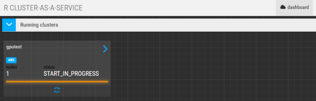
I deployed a one-node cluster on Teraproc.com using the Amazon g2.2xlarge machine type as shown below. I could have installed the g2.2xlarge instance myself from the Amazon EC2 console, but in this case I would have needed to install R, R Studio and configure the environment myself resulting in spending more time and money. You can learn how to set up an R cluster yourself on different node types (including free machines) at the Teraproc R Analytics Cluster-as-a-Service website. If you already have an Amazon EC2 account you can set up a cluster in as little as five minutes.
The g2.2xlarge machine instance is a Sandy Bridge based machine with 8 cores / vCPUs on a Xeon E5-2670 processor, 15GB or memory, a solid state disk drive and an NVIDIA GRID K520 GPU. The on-demand price for this machine is $0.65 per hour. The NVIDIA GRID K520 has two GK104 graphics processors each with 1,536 cores on a single card with 8 GB of RAM.
Running Our Example
First we use the teraproc.com R-as-a-cluster service to provision the R environment making sure that we select the correct machine type (G22xlarge) and install a one-node cluster, as Figure 1 shows. This automatically deploys a single-node cluster complete with R Studio and provides us with a URL to access the R Studio environment.
Using the shell function within R Studio (under the Tools menu), I can run an operating system command to make sure that the GPU is present on the machine.
gordsissons@ip-10-0-93-199:~$ lspci | grep -i nvidia
00:03.0 VGA compatible controller: NVIDIA Corporation GK104GL [GRID K520] (rev a1)
To use the rpud package to access GPU functions we need to install it first. Run the command below from inside R-Studio to install rpud from CRAN.
> install.packages(“rpud”)
Next, use the library command to access rpud functions.
> library(rpud)
Rpudplus 0.5.0
http://www.r-tutor.com
Copyright (C) 2010-2015 Chi Yau. All Rights Reserved.
Rpudplus is free for academic use only. There is absolutely NO warranty.
If everything is working properly, we should be able to see the GPU on our Amazon instance from the R command prompt by calling rpuGetDevice.
> rpuGetDevice()
GRID K520 GPU
[1] 0
The following listing shows a sample R program that compares performance of a hierarchical clustering algorithm with and without GPU acceleration. The first step is to create a suitable dataset where we can control the number of observations (rows) as well as the number of dimensions (columns) for each observation. The test.data function returns a matrix of random values based on the number of rows and columns provided.
The run_cpu function calculates all the distances between the observations (rows) using R’s dist function, and then runs R’s native hclust function against the computed distances stored in dcpu to create a dendrogram. The run_gpu function performs exactly the same computations using the GPU-optimized versions of dist and hclust (rpuDist and rpuHclust<em>) from the rpud package.
The R script creates a matrix m of a particular size by calling test.data and then measures and displays the time required to create a hierarchical cluster using both the CPU and GPU functions.
library("rpud")
#
# function to populate a data matrix
#
test.data <- function(dim, num, seed=10) {
    set.seed(seed)
    matrix(rnorm(dim * num), nrow=num)
}

run_cpu <- function(matrix) {
    dcpu <- dist(matrix)
    hclust(dcpu)
}

run_gpu <- function(matrix) {
    dgpu <- rpuDist(matrix)
    rpuHclust(dgpu)
}

#
# create a matrix with 20,000 observations each with 100 data elements
#
m <- test.data(100, 20000)

#
# Run dist and hclust to calculate hierarchical clusters using CPU
#

print("Calculating hclust with Sandy Bridge CPU")
print(system.time(cpuhclust <-run_cpu(m)))

#
# Run dist and hclust to calculate hierarchical clusters using GPU
#

print("Calculating hclust with NVIDIA K520 GPU")
print(system.time(gpuhclust <- run_gpu(m)))
Running the script yields the following results:
>source('~/examples/rgpu_hclust.R')
[1] "Calculating hclust with Sandy Bridge CPU"
user     system elapsed
294.760   0.746 295.314
[1] "Calculating hclust with NVIDIA K520 GPU"
user     system elapsed
19.285    3.160  22.431
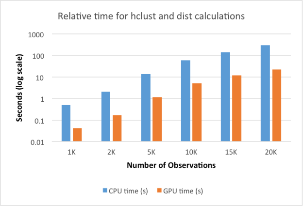
To explore the GPU vs. CPU speedup, we ran the script on datasets with a varying number of rows and plotted the results. The distance calculation is highly parallel on the GPU, while much of the GPU-optimized hclust calculation runs on the CPU. For this reason the calculation scales well as the dataset gets larger and the time required for the distance calculations dominates.
| Number of rows | Number of dimensions | Total elements | # distance calculations | CPU time (seconds) | GPU time (seconds) | Speed-up |
| 1,000 | 100 | 100,000 | 1,998,000 | 0.50 | 0.04 | 11.8 |
| 2,000 | 100 | 200,000 | 7,996,000 | 2.06 | 0.17 | 12.1 |
| 5,000 | 100 | 500,000 | 49,990,000 | 13.42 | 1.17 | 11.5 |
| 10,000 | 100 | 1,000,000 | 199,980,000 | 59.83 | 5.03 | 11.9 |
| 15,000 | 100 | 1,500,000 | 449,970,000 | 141.15 | 11.61 | 12.2 |
| 20,000 | 100 | 2,000,000 | 799,960,000 | 295.31 | 22.43 | 13.2 |
Looking at the run times side by side, we see that running the multiple steps with the GPU is over ten times faster than running on the CPU alone.
The result of our analysis is a hierarchical cluster that we can display as a dendrogram like Figure 1 using R’s plot command.
> plot(gpuhclust,hang = -1)
Conclusion
Our results clearly show that running this type of analysis on a GPU makes a lot of sense. Not only can we complete calculations ten times faster, but just as importantly we can reduce the cost of resources required to do our work. We can use these efficiencies to do more thorough analysis and explore more scenarios. By using the Teraproc service, we make GPU computing much more accessible to R programmers who may not otherwise have access to GPU-capable nodes.
In a future post we’ll show how you can tackle very large analysis problems with clusters of GPU-capable machines. Try out Teraproc R Analytics Cluster-as-a-Service today! To learn about other ways to accelerate your R code with GPUs, check out the post Accelerate R Applications with CUDA by NVIDIA’s Patric Zhao.