
The average car contains over 100 sensors to both monitor and respond to vital information. Ranging from an overheating engine to low tire pressure and erratic steering, sensors exist to provide automatic data, insight, and control. They make the act of driving safer for both the passengers and everyone else on the road. Of course, sensors aren’t limited to cars.
Your local airport’s radar system tracks airplanes and other large objects, guiding flights safely into the air and to the ground. The cell phone in your pocket uses its on-device radio and antenna to send your voice over the ether to a friend located in a different country, free of noise or interference. A surgeon uses real-time inner cavity camera feeds to detect anomalies, identify diseased tissues, and classify legions.
In each case, sensors collect information from the environment while computers analyze and process the resulting data stream. The results of real-time processing and analysis are either used to provide feedback to a human operator or to close a control loop automatically.
Challenges with building sensor-processing applications
Traditional sensor processing systems are hardware-defined and are often tightly coupled with the frontend sensor. A modification of either the sensor, computer, or pre-existing application could potentially require non-trivial upgrades across the entire application framework.
For example, if you’re running an application on a framework designed for real-time computer vision tasks, it’s often challenging to add other data sources easily, such as voice, as application goals expand.
Augmenting an existing sensor processing application with an AI inferencing model can be even more challenging as you may have to learn new tools and software libraries, and how to optimize for real-time streaming performance.
NVIDIA Holoscan overview
NVIDIA Holoscan is a real-time, low-latency, and sensor-agnostic software development kit to prototype, build, deploy, and scale streaming sensor applications. First introduced for medical AI use cases, Holoscan is now being used for a broader range of applications across multiple industries for high performance computing at the edge. With Holoscan, a C++ or Python developer builds a connected graph of relevant nodes, called operators, to define an application.
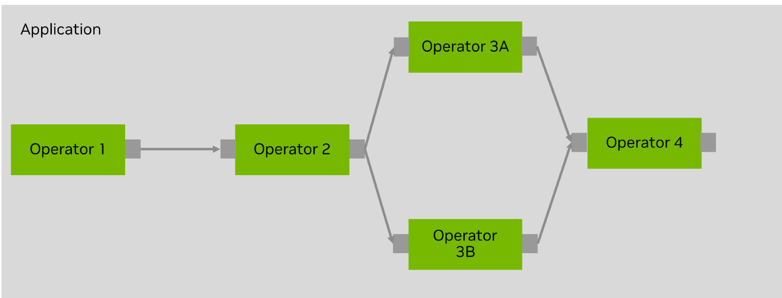
These operators are flexible, straightforward to program or modify, and consist of isolated and commonly used tasks. For example, a network operator could be used to facilitate the ingestion of a UDP Ethernet packet directly to GPU without engaging the CPU. Another operator could perform AI inferencing, such as an NVIDIA TensorRT-optimized YOLO object detector. A final operator could perform a GPU-accelerated FFT in C++ with cuFFT.
When the operators are implemented, you specify how data connects into and out of them. The operators can then be saved for future use by another application pipeline.
Holoscan abstracts away data movement and provides a set of simple APIs to build applications with existing NVIDIA SDKs on top of high-speed sensor data. Holoscan enables you to build end-to-end, multi-modal, AI-driven, software pipelines from multiple sensor domains.
For more information about Holoscan, particularly the features introduced in the current Holoscan SDK v0.4 release, see Rapidly Building Streaming AI Apps with Python and C++ Holoscan.
Reference applications for radio, radar, and more with HoloHub
HoloHub is a new GitHub repository that hosts reference Holoscan applications and operators. HoloHub is designed to be a comprehensive, rich collection of pre-built operators. It includes examples and end-to-end applications of how to use and scale them. We welcome contributions!
In addition to reference applications published as part of Holoscan SDK v0.4, here are the first two reference applications published on HoloHub, both written in Python:
- SDR FM Demodulation Application: FM demodulation with software-defined radio (SDR)
- Simple Radar Pipeline Application: Traditional radar signal-processing pipeline
While these examples focus on the Holoscan Python API, the C++ example closely follows the same syntax and design principles. One driving philosophy of Holoscan is that both data scientists and performance engineers can work together on the same underlying framework, C++-based Holoscan.
Here are some examples to show you how to build and deploy Holoscan pipelines.
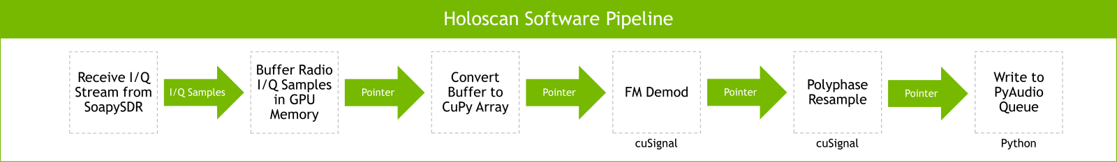
Software-defined radio: FM demodulation
We’re all familiar with a car’s radio; you move a rotary dial to tune to your favorite station and then crank up the volume! The radio is using hardware elements to do analog decoding from radio waves to voice. With the advent of SDR, like the inexpensive RTL-SDR, you now have a mechanism to implement what used to be a hardware-defined problem with software.
Software-based FM demodulation, also known as listening to the radio) is the “Hello World” example of signal-processing applications. Many beginning developers have learned to program accelerators with it. Due to its relative simplicity, FM demodulation serves as a quick check that you can capture radio waves with SDR and then demodulate and play back the results in real time.
In this Holoscan example, you use an RTL-SDR USB dongle along with the SoapySDR driver to collect, stream, and buffer complex-valued radio samples. This data is then passed to an FM demodulation and resampling operator that uses cuSignal. The demodulated output is then placed in a Python queue, which triggers playback through PyAudio.
A Holoscan application consists first of an Application class where off-the-shelf and custom operators are defined, along with how they connect to one another. The following code example shows the FMDemod Application class:
class FMDemod(Application):

   def __init__(self):
  	super().__init__()

   def compose(self):
  	src = SignalGeneratorOp(self, CountCondition(self, 500), name="src")
  	demodulate = DemodulateOp(self, name="demodulate")
  	resample = ResampleOp(self, name="resample")
  	sink = SDRSinkOp(self, name="sink")

   self.add_flow(src, demodulate)
   self.add_flow(demodulate, resample)
   self.add_flow(resample, sink)
The compose function of the Application class is used to define operators used in the Holoscan pipeline. In this example, there are four custom operators:
SignalGeneratorOp: Brings complex-valued tensor data from SDR to GPU and exposes it to Holoscan.DemodulateOp: Performs FM demodulation on incoming data with cuSignal.ResampleOp: Downsamples the SDR sample rate to 48 kHz, that of computer audio output for playback with cuSignal.SDRSinkOp: Connects to PyAudio for real-time audio playback.
The source operator, SignalGeneratorOp, includes an additional parameter that controls the scheduling and runtime of the source node within a Holoscan graph. The CountCondition option runs the source for a given number of times (in this case, 500). There are additional scheduling options discussed in the Holoscan documentation that run a given source node until toggled, such as BinaryCondition.
Operators are connected, creating a graph, with add_flow(<input>, <output>).
In this example, these operators are connected in a linear fashion:
SignalGeneratorOpoutput feedsDemodulateOp.DemodulateOpoutput feedsResampleOp.ResampleOpoutput feedsSDRSinkOp.
Custom operators are based on the Operator Holoscan class and consist of the following major functions:
__init__: Defines parameters used within the custom operator.setup: Defines a custom operator’s input and output connections.compute: Performs data transformation, compute, or connect to an external library.
To better understand how to build a custom operator, here’s DemodulateOp in more detail.
Class DemodulateOp(Operator):

   def __init__(self, *args, **kwargs):
  	# Need to call the base class constructor last
  	super().__init__(*args, **kwargs)

   def setup(self, spec: OperatorSpec):
  	spec.input(“rx_sig”)
  	spec.output("sig_out")

   def compute(self, op_input, op_output, context):
  	sig = op_input.receive("rx_sig")
  	print("In Demodulate – Got: ", sig[0:10])
  	op_output.emit(uSignal.fm_demod(sig), "sig_out")
In this example, the setup function defines the operator input and output ports. In this case, there is one stream of data entering the operator and one leaving.
The bulk of the work performed in the operator is done in the compute function. Here, you can access and manipulate incoming data through op_input.receive(<name_of_input>) and run some type of operation on that data. In this case, I am using uSignal’s fm_demod function to perform an FM demodulation. Upon completion, you output the results with op_output.emit(<data>, <name_of_output>).
Simple radar signal-processing pipeline
Radar systems were first developed during World War II to help detect and track enemy aircraft. They were instrumental to the Allied powers’ success in the Battle of Britain.
Straightforward in concept, radar works by transmitting a known signal and waiting for that signal to bounce off an object and return to the receiver. The time delta and position are considered, along with other signal-processing techniques, to measure a target’s position and speed.
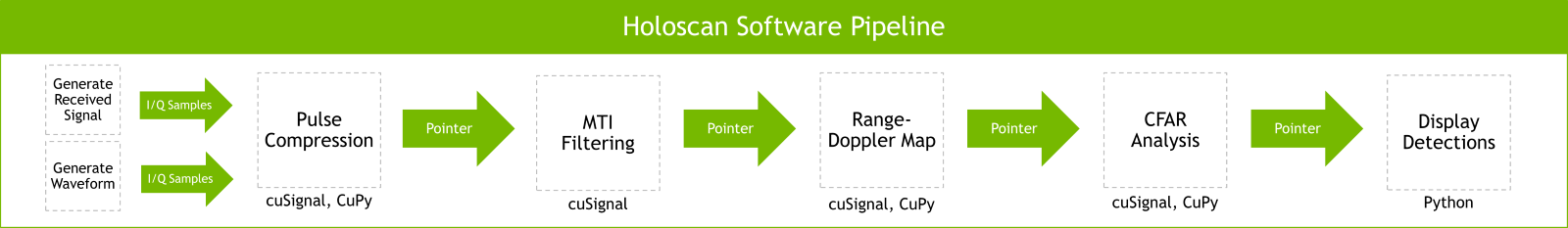
Here, a generated waveform is matched filtered with a received signal to determine if the transmitted signal was received. From there, you perform various filtering operations to remove stationary or slow-moving objects, called clutter, and increase resolution. Finally, you analyze the detection targets and display candidate positions on the screen.
In this Holoscan example, you are generating streaming data on the fly with CuPy in the source operator, but you could easily leverage a network operator to ingest UDP Ethernet. Like the FM demodulation example earlier, cuSignal and CuPy are used to build the application-specific operators.
Unlike the FM demodulation example, this Holoscan pipeline contains operators that have multiple inputs and outputs. The following code example shows how this is implemented in Python. Multiple inputs are specified in the setup function, and the associated data object can be accessed in the compute function through op_input.receive(<name_of_input>).
class PulseCompressionOp(Operator):

   def __init__(self, *args, **kwargs):
  	super().__init__(*args, **kwargs)

   def setup(self, spec: OperatorSpec):
  	spec.input("x")
  	spec.input("waveform")
  	spec.output("X")

   def compute(self, op_input, op_output, context):
  	x = op_input.receive("x")
  	waveform = op_input.receive("waveform")
<code omitted for brevity>
Next steps
The FM demodulation and radar examples don’t currently include an AI Inferencing step. However, the flexibility of Holoscan enables you to add a new operator to an existing graph without negatively impacting application performance or its maintainability.
While the radar pipeline is currently offline and uses simulated data, you could add a network operator, as previously discussed, without negatively impacting the rest of the compute pipeline. For more information about reference applications with AI inferencing and real-time data ingestion, see NVIDIA Holoscan SDK v0.4.
To learn more about building streaming AI pipelines for a variety of domains, join the Holoscan Developer Day and training lab at NVIDIA GTC on Building High-Speed Sensor AI Pipelines using NVIDIA Holoscan. GTC, the developer conference for the era of AI and the metaverse, is free to attend and takes place March 20–23.
