Accelerating SE(3)-Transformers Training Using an NVIDIA Open-Source Model Implementation

SE(3)-Transformers are versatile graph neural networks unveiled at NeurIPS 2020. NVIDIA just released an open-source optimized implementation that uses 43x less memory and is up to 21x faster than the baseline official implementation.

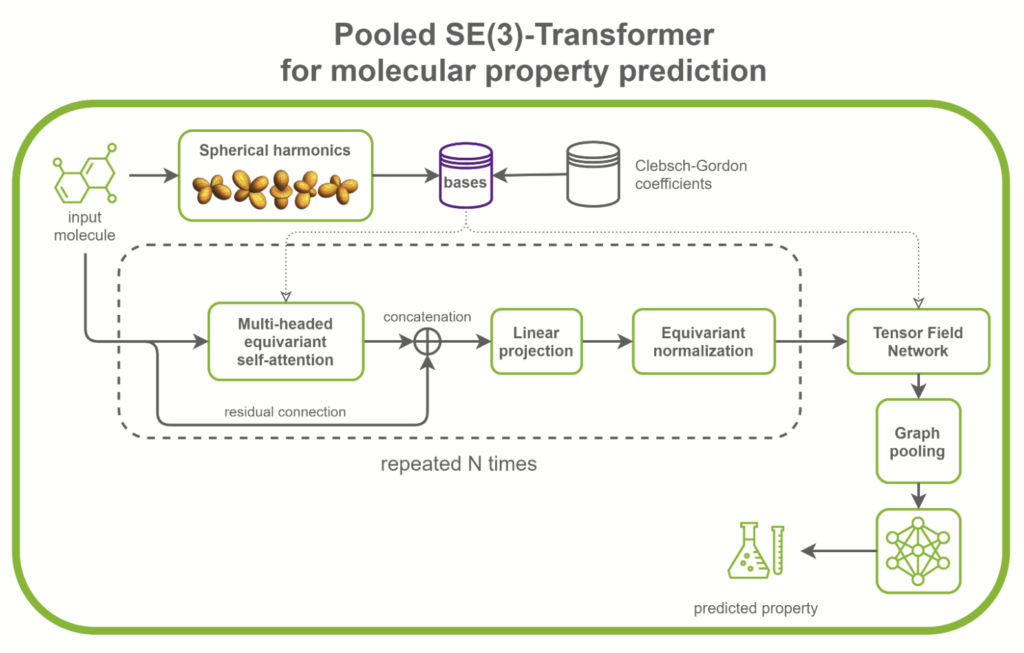
SE(3)-Transformers are useful in dealing with problems with geometric symmetries, like small molecules processing, protein refinement, or point cloud applications. They can be part of larger drug discovery models, like RoseTTAFold and this replication of AlphaFold2. They can also be used as standalone networks for point cloud classification and molecular property prediction (Figure 1).

In the /DGLPyTorch/DrugDiscovery/SE3Transformer repository, NVIDIA provides a recipe to train the optimized model for molecular property prediction tasks on the QM9 dataset. The QM9 dataset contains more than 100k small organic molecules and associated quantum chemical properties.

A 21x higher training throughput

The NVIDIA implementation provides much faster training and inference overall compared with the baseline implementation. This implementation introduces optimizations to the core component of SE(3)-Transformers, namely tensor field networks (TFN), as well as to the self-attention mechanism in graphs.

These optimizations mostly take a form of fusion of operations, given that some conditions on the hyperparameters of attention layers are met.

Thanks to these, the training throughput is increased by up to 21x compared to the baseline implementation, taking advantage of Tensor Cores on recent NVIDIA GPUs.

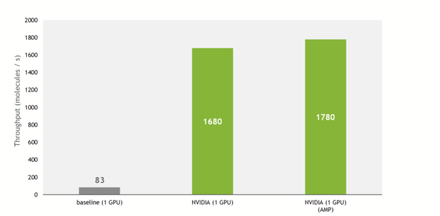
Training throughput in molecules per second: baseline: 83, NVIDIA: 1680, NVIDIA with AMP: 1780. — *Figure 2. Training throughput on an A100 GPU. QM9 dataset with a batch size of 100.*

In addition, the NVIDIA implementation allows the use of multiple GPUs to train the model in a data-parallel way, fully using the compute power of a DGX A100 (8x A100 80GB).

Putting everything together, on an NVIDIA DGX A100, SE(3)-Transformers can now be trained in 12 minutes on the QM9 dataset. As a comparison, the authors of the original paper state that the training took 2.5 days on their hardware (NVIDIA GeForce GTX 1080 Ti).

Faster training enables you to iterate quickly during the search for the optimal architecture. Together with the lower memory usage, you can now train bigger models with more attention layers or hidden channels, and feed larger inputs to the model.

A 43x lower memory footprint

SE(3)-Transformers were known to be memory-heavy models, meaning that feeding large inputs like large proteins or many batched small molecules was challenging. This was a bottleneck for users with limited GPU memory.

This has now changed with the NVIDIA implementation, open-sourced on DeepLearningExamples. Figure 3 shows that, thanks to NVIDIA optimizations and support for mixed precision, the training memory usage is reduced by up to 43x compared to the baseline implementation.

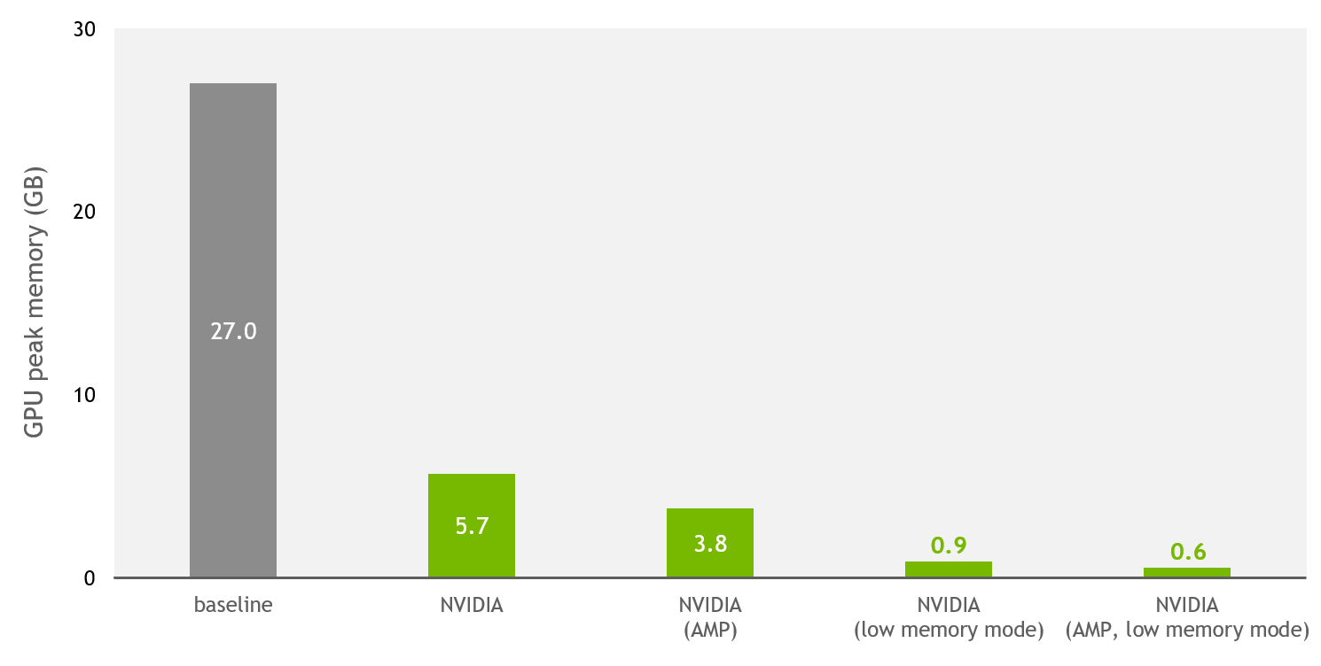
Peak memory usage: baseline: 27 GB, NVIDIA: 5.7 GB; NVIDIA with AMP: 3.8 GB; NVIDIA with low-memory mode: .9 GB; NVIDIA with AMP and low-memory mode: .6 GB. — Figure 3. Comparison of training peak memory consumption between the baseline implementation and NVIDIA implementation of SE(3)-Transformers. Using 100 molecules per batch on the QM9 dataset. V100 32-GB GPU.

In addition to the improvements done for single and mixed precision, a low-memory mode is provided. When this flag is enabled, and the model runs either on TF32 (NVIDIA Ampere Architecture) or FP16 (NVIDIA Ampere Architecture, NVIDIA Turing Architecture, and NVIDIA Volta Architecture) precisions, the model switches to a mode that trades throughput for extra memory savings.

In practice, on the QM9 dataset with a V100 32-GB GPU, the baseline implementation can scale up to a batch size of 100 before running out of memory. The NVIDIA implementation can fit up to 5000 molecules per batch (mixed precision, low-memory mode).

For researchers handling proteins with amino acid residue as nodes, this means that you can feed longer sequences and increase the receptive field of each residue.

SE(3)-Transformer optimizations

Here are some of the optimizations that the NVIDIA implementation provides compared to the baseline. For more information, see the source code and documentation on the /DGLPyTorch/DrugDiscovery/SE3Transformer repository.

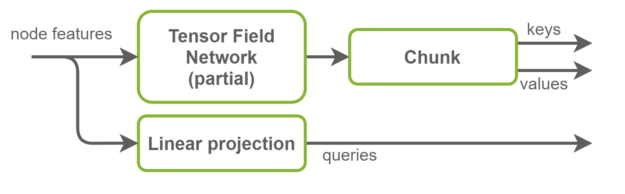
Fused keys and values computation

Inside the self-attention layers, keys, queries, and values tensors are computed. Queries are graph node features and are a linear projection of the input features. Keys and values, on the other hand, are graph edge features. They are computed using TFN layers. This is where most computation happens in SE(3)-Transformers and where most of the parameters live.

The baseline implementation uses two separate TFN layers to compute keys and values. In the NVIDIA implementation, those are fused together in one TFN with the number of channels doubled. This reduces by half the number of small CUDA kernels launched, and better exploits GPU parallelism. Radial profiles, which are fully connected networks inside TFNs, are also fused with this optimization. An overview is shown in Figure 4.

Block diagram of keys, queries, and values computation. — *Figure 4. Keys, queries, and values computation inside the NVIDIA implementation. Keys and values are computed together and then chunked along the channel dimension.*

Fused TFNs

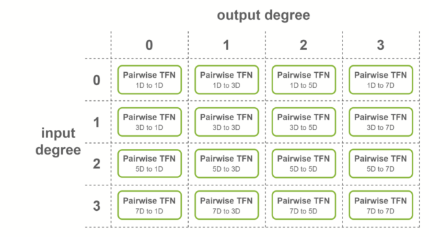
Features inside SE(3)-Transformers have, in addition to their number of channels, a degree $d$ , which is a positive integer. A feature of degree $d$ has a dimensionality $2d + 1$ . A TFN takes in features of different degrees, combines them using tensor products, and outputs features of different degrees.

For a layer with 4 degrees as input and 4 degrees as output, all combinations of degrees are considered: there are in theory 4×4=16 sublayers that must be computed.

These sublayers are called pairwise TFN convolutions. Figure 5 shows an overview of the sublayers involved, along with the input and output dimensionality for each. Contributions to a given output degree (columns) are summed together to obtain the final features.

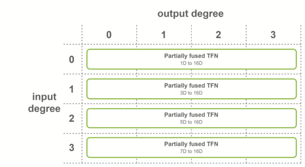
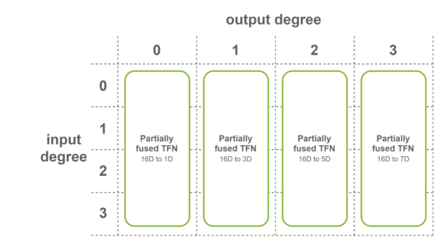
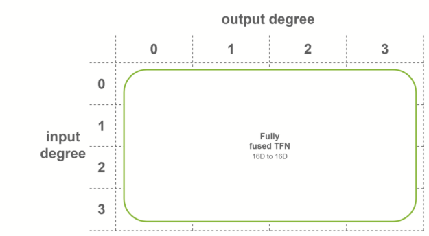
4 by 4 grid of all pairwise TFN convolutions. — *Figure 5. Pairwise convolutions involved in a TFN layer with 4 degrees as input and 4 degrees as output.*

NVIDIA provides multiple levels of fusion to accelerate these convolutions when some conditions on the TFN layers are met. Fused layers enable Tensor Cores to be used more effectively by creating shapes with dimensions being multiples of 16. Here are three cases where fused convolutions are applied:

Output features have the same number of channels
Input features have the same number of channels
Both conditions are true

The first case is when all the output features have the same number of channels, and output degrees span the range from 0 to the maximum degree. In this case, fused convolutions that output fused features are used. This fusion level is used for the first TFN layer of SE(3)-Transformers.

1 by 4 grid of 4 fused convolutions — *Figure 6. Partially fused TFN per output degree.*

The second case is when all the input features have the same number of channels, and input degrees span the range from 0 to the maximum degree. In this case, fused convolutions that operate on fused input features are used. This fusion level is used for the last TFN layer of SE(3)-Transformers.

4 by 1 grid of 4 fused convolution — *Figure 7. Partially fused TFN per input degree.*

In the last case, fully fused convolutions are used when both conditions are met. These convolutions take as input fused features, and output fused features. This means that only one sublayer is necessary per TFN layer. Internal TFN layers use this fusion level.

single fully fused convolution — *Figure 8. Fully fused TFN*

Base precomputation

In addition to input node features, TFNs need basis matrices as input. There exists a set of matrices for each graph edge, and these matrices depend on the relative positions between the destination and source nodes.

In the baseline implementation, these matrices are computed in the beginning of the forward pass and shared across all TFN layers. They depend on spherical harmonics, which can be expensive to compute. Because the input graphs do not change (no data augmentation, no iterative position refinement) with the QM9 dataset, this introduces redundant computation across epochs.

The NVIDIA implementation provides the option to precompute those bases at the beginning of the training. The full dataset is iterated one time and the bases are cached in RAM. The process of computing bases at the beginning of forward passes is replaced by a faster CPU to GPU memory copy.

Conclusion

I encourage you to check the implementation of the SE(3)-Transformer model in the NVIDIA /DGLPyTorch/DrugDiscovery/SE3Transformer GitHub repository. In the comments, share how you plan to adopt and extend this project.