Accelerating Random Forests Up to 45x Using cuML

This post was originally published on the RAPIDS AI blog.

Random forests are a popular machine learning technique for classification and regression problems. By building multiple independent decision trees, they reduce the problems of overfitting seen with individual trees.

In this post, I review the basic random forest algorithms, show how their training can be parallelized on NVIDIA GPUs, and finally present benchmark numbers demonstrating the performance. For more information about the random forests algorithm, see An Implementation and Explanation of the Random Forest in Python (Toward Data Science) or Lesson 1: Introduction to Random Forests (Fast.ai).

*Figure 1. Example random forest with three decision trees.*

Random forests

The main idea behind random forests is to learn multiple independent decision trees and use a consensus method to predict the unknown samples. Additionally, random forests use the techniques of bagging and feature subsampling to make sure that no two resulting decision trees are the same.

With bagging (bootstrap aggregation), each decision tree is trained upon a different sample, with the replacement of the original dataset. In this bootstrapped dataset, a given sample, or row, of the training data can exist multiple times due to replacement.

When the algorithm decides on a split during tree building, only a random sample of features or columns, without replacement, is considered. Feature subsampling can highlight different aspects of the dataset that might go unnoticed if overpowered by more prominent features.

Training

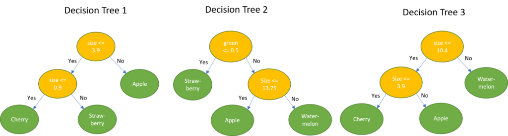
The following example is a small classification dataset of fruits, based on their physical appearance. Assume that you want to build a random forest containing three trees to classify different fruits in this dataset.

Instance	Red	Green	Blue	Size (cm)	Fruit (Label)
0	1.0	0.0	0.0	7.0	Apple
1	0.0	1.0	0.0	20	Water Melon
2	1.0	0.0	0.0	1.0	Cherry
3	0.0	1.0	0.0	7.5	Apple
4	1.0	0.0	0.0	1.0	Strawberry
5	1.0	0.0	0.0	0.8	Cherry

view raw fruit_rf_training.csv hosted with ❤ by GitHub

The first step is to create three datasets, one for each tree, after applying bagging with replacement and feature subsampling without replacement on this input dataset. In this toy dataset, I’m not demonstrating feature subsampling due to its small size.

Instance	Red	Green	Blue	Size (cm)	Fruit (Label)
5	1.0	0.0	0.0	0.8	Cherry
0	1.0	0.0	0.0	7.0	Apple
0	1.0	0.0	0.0	7.0	Apple
4	1.0	0.0	0.0	1.0	Strawberry

view raw fruit_subsampled_dataset_1.csv hosted with ❤ by GitHub

Dataset 1

Instance	Red	Green	Blue	Size (cm)	Fruit (Label)
4	1.0	0.0	0.0	1.0	Strawberry
4	1.0	0.0	0.0	1.0	Strawberry
1	0.0	1.0	0.0	20	Water Melon
3	0.0	1.0	0.0	7.5	Apple

view raw fruit_subsampled_dataset_2.csv hosted with ❤ by GitHub

Dataset 2

Instance	Red	Green	Blue	Size (cm)	Fruit (Label)
1	0.0	1.0	0.0	20	Water Melon
0	1.0	0.0	0.0	7.0	Apple
5	1.0	0.0	0.0	0.8	Cherry
2	1.0	0.0	0.0	1.0	Cherry

view raw fruit_subsampled_dataset_3.csv hosted with ❤ by GitHub

Dataset 3

After this, you build three independent decision trees using each of these subsampled datasets. The tree-building algorithm is covered in detail in the next section.

Inference

To infer the output class for classification problems or predict the output for regression problems of a previously unknown input sample, the sample is passed through every decision tree in the forest and individual tree predictions are noted. In the case of classification, the output class label is decided based on the majority vote of all decision trees. In the case of regression, the prediction is the mean of all individual tree predictions.

Taking the example fruit dataset as an example, the goal now is to determine the name of the fruit, given a new measurement.

Example 1: {0.0, 1.0, 0.0, 18cm}. This sample has 1.0 for the green color and 18 as size. Classifying this using the decision trees leads to the following result:

majority{Apple, Watermelon, Watermelon} = Watermelon

Example 2: {1.0, 0.0, 0.0, 1cm}. This sample has 1.0 for the color red and 1cm as size. Classifying this using the decision trees leads to the following result:

majority{Strawberry, Strawberry, Cherry} = Strawberry

*Figure 2. Three fruit decision trees showing pure nodes.*

Decision tree algorithm

Because random forests are a collection of decision trees, they need to start with an efficient algorithm to build a single tree.

Finding splits

Finding the best split at a particular node involves two choices: choosing the feature and split value for that feature that will result in the highest improvement to the model. The datasets sent to each of the two children of this node should have lower impurity than the parent node. That is, the examples within each node should have outcomes that are as similar to each other as possible.

Splitting nodes continues until either all values in the subset mapping to that node are pure (for example, all fruits are strawberries) or some other conditions are met (for example, maximum tree depth, maximum number of samples per tree node).

At each node, the algorithm uses a specified metric to estimate how much a potential split improves the model. cuML supports a number of split goodness metrics. For classification, either Gini Impurity or Entropy is used, while for regression either Mean Squared Error (MSE) or Mean Absolute Error (MAE). You can specify which metric to use, such as the split_criterion option in Python. However, for most users, it’s not critical to know the details of these metrics and the default works well.

Assume that you are using the Gini Impurity metric to decide how to split a tree node. A potential split S, defined by feature split_value, splits this node’s dataset of N rows into left and right subsets with N_left and N_right rows, respectively. The improvement of split S is computed with the following equations:

improvement = Giniᴾᴬᴿᴱᴺᵀ — impurity

impurity = N_left/N * Giniᴸᵉᶠᵗ + N_right/N * Giniᴿⁱᵍʰᵗ

The algorithm computes the potential improvement of many potential splits for all the features, and selects the split that yields the maximum information gain. Because the number of split options is so large, only a subset of potential split values is considered per feature.

Accelerating the split calculation with quantiles and histograms

The cuML Random Forest model contains two high-performance split algorithms to select which values are explored for each feature and node combination: min/max histograms and quantiles.

In both cases, at most n_bins split values are considered per feature. You can specify which split algorithm to use (split_algo option in Python), as well as the number of bins (n_bins option). These approaches draw inspiration from the algorithm used in GPU-accelerated XGBoost and greatly reduce the work needed for split computation relative to an exhaustive search.

Min/max histograms: A histogram is built for every feature for a tree node. Every feature’s data range [min, max] is split into n_bins equally sized bins. The end range of each bin is considered as a potential split value. With this approach, the split values for each feature are recomputed at each node, thus adapting to the data ranges at each tree node. The min/max algorithm also helps in isolating outliers in the data at an early stage during the tree building process.
Quantiles: The quantiles split algorithm precomputes the potential split values for each feature one time per tree, at the root node. Each feature column is sorted in ascending order, and split into n_bins such that each bin contains an equal portion of the root node’s dataset. The end range of each bin is considered as a potential split value.

Unlike min/max histograms where all bins have the same width, in quantiles, all bins, except for the last one, have the same height for the root note but are of variable width. As split values are precomputed one time per tree, the quantile approach is faster than the min/max histogram algorithm. If, for a node deep in the tree, all feature values fall under a single bin, then no splitting can take place for that feature. A further optimization supported with the quantile_per_tree Python option is to compute the split values one time per random forest, that is, for the original non-bootstrapped dataset, rather than one time per decision tree.

Leaf nodes

A regular, non-leaf, decision tree node holds a split condition such as feature split_value, but a leaf tree node holds a prediction. If the leaf node is not pure—it contains samples with different target feature values, the prediction is computed as follows:

For classification, the prediction is the label appearing more often, or one of them in case of a tie.
For regression, the prediction is the arithmetic mean of all target values.

Building decision trees: putting it all together

Building individual decision trees is where the heavy lifting of the random forest is done. Individual trees are built using a list of bootstrapped samples, as discussed earlier. Many algorithms use a top-down approach, proceeding with depth-first splits of each node and then each newly created child node. In a GPU context, this can lead to launching an enormous number of CUDA kernels, one per node. These small kernels quickly get queued up as launch time begins to dominate the processing.

To remove this bottleneck, cuML uses a breadth-first algorithm, building a full layer of the tree at a time. This makes the runtime of the algorithm scale roughly linearly with depth. The decision tree building process has a simple structure:

	(A) Initialize a bit mask indicating which samples are contained in each node
	(B) Initialize a “node map” indicating which nodes are present at each level
	(C) ForEach(tree_level)
	1. Find the node id of all data samples, using the bit mask
	2. Compute the possible splits for all bins, all columns and all nodes
	3. Find the best split for each node
	4. Update the bit mask and sparse node map to feed the next level

view raw pseudo_code hosted with ❤ by GitHub

Building forests across multiple GPUs

cuML recently added an experimental feature to take this parallelism one step further and construct trees in parallel across multiple GPUs on the same node or across a cluster. This approach builds on the Dask distributed processing library.

In the distributed random forest approach, you first use Dask to distribute the training data to all worker GPUs and then fit a cuml.dask.ensemble.RandomForestClassifier object. The data can be randomly split and shared equally across all workers, in which case each worker builds trees on a subset of the full data. Alternatively, training data can be replicated so that each worker has a complete view of the dataset. In practice, the random sharing approach effectively expands the amount of available memory and typically works well. However, it may slightly reduce model accuracy.

For a random forest with T trees and W workers, each worker builds T/W trees on its 1/Wᵗʰ fraction of locally available data. As little communication is required, random forests can scale efficiently to many GPUs. At inference time, predictions from trees on all of the workers are combined, just as if the trees had all been trained on a single GPU.

The Dask RF features in cuML are still experimental, and the API is subject to change in future releases. But it’s a great chance to check out the future of distributed RF and see how it works for your application.

Example: side-by-side single GPU RF with scikit-learn

As with other modules in cuML, the random forest implementation follows the scikit-learn API closely. Instantiate a random forest object and then call the fit and predict methods.

    |  ######cuML######                 |  ######Sklearn######                 |
|                                   |                                      |
|  from cuml import                 |  from sklearn.ensemble import        |
|  RandomForestClassifier as cuRF   |  RandomForestClassifier as sklRF     |
|                                   |  import multiprocessing as mp        |
|                                   |                                      |
|  # cuml Random Forest params      |  #sklearn Random Forest params       |
|  cu_rf_params = {                 |  skl_rf_params = {                   |
|     ‘n_estimators’: 25,           |      ‘n_estimators’: 25,             |
|     ‘max_depth’: 13,              |      ‘max_depth’: 13,                |
|      ‘n_bins’: 15,                |                                      |
|      ‘n_streams’: 8 }             |      ‘n_jobs’: mp.cpu_count() }      |
|                                   |                                      |
|  cu_rf = cuRF(**cu_rf_params)     |  skl_rf = sklRF(**skl_rf_params)     |
|  cu_rf.fit(X_train, y_train)      |  skl_rf.fit(X_train, y_train)        |
|                                   |                                      |
|  print("cuml RF Accuracy Score: " |  print("sklearn RF Accuracy Score: " |
|  accuracy_score(                  |  accuracy_score(                     |
|  cu_rf.predict(X_test), y_test))  |  skl_rf.predict(X_test), y_test))    |


  

view raw sidebyside.markdown hosted with ❤ by GitHub

Example: Building on multiple GPUs with Dask

Parallelizing to multiple GPUs with the experimental Dask interface is straightforward. This approach starts by distributing the data evenly across all the workers and then fits a cuml.dask.ensemble.RandomForestClassifier object.

	from cuml.dask.ensemble import RandomForestClassifier as cuRF_mg
	# cuml Random Forest params
	cu_rf_params = {
	‘n_estimators’: 25,
	‘max_depth’: 13,
	‘n_bins’: 15,
	‘n_streams’: 8
	}

	# Start by setting up the CUDA cluster on the local host
	cluster = LocalCUDACluster(threads_per_worker=1, n_workers=n_workers)
	c = Client(cluster)
	workers = c.has_what().keys()

	# Shard the data across all workers
	X_train_df, y_train_df = dask_utils.persist_across_workers(c,[X_train_df,y_train_df],workers=workers)

	# Build and train the model
	cu_rf_mg = cuRFC_mg(**cu_rf_params)
	cu_rf_mg.fit(X_train_df, y_train_df)

	# Check the accuracy on a test set
	cu_rf_mg_predict = cu_rf_mg.predict(X_test)
	acc_score = accuracy_score(cu_rf_mg_predict, y_test, normalize=True)
	c.close()
	cluster.close()

view raw mg_rf_dask.py hosted with ❤ by GitHub

Benchmarks

To show the performance speedups, my team and I ran some benchmark tests for single GPU and multi-GPU with Dask.

Single GPU

Start by looking at the performance of random forest training in cuML compared with sklearn. In the following tests, we used the release branch-0.10 for cuML and version 0.21.2 for sklearn, running on an NVIDIA DGX-1 server with eight V100–16GB GPUs and dual Xeon E5–2698v4@2.20GHz CPUs with 40 CPU cores in total. We used one V100–16GB GPU for single-GPU cuML runs and the maximum number of threads available, that is, 80 CPU threads on the DGX-1 server, for sklearn runs. To ensure the best performance, we used a GPU dataframe as input to cuML and a numpy array as input to sklearn.

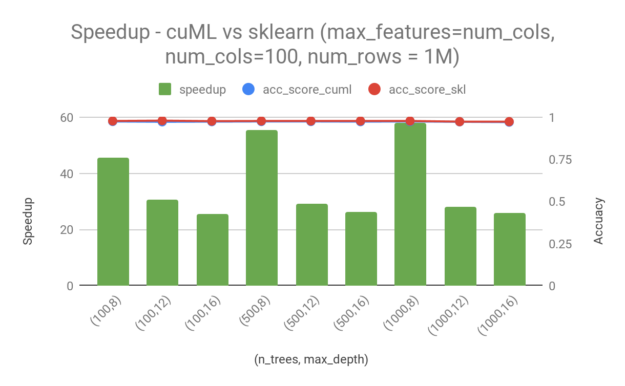
To analyze the performance in a real-world scenario, we trained models on the Higgs dataset, which has 28 columns and 11M rows. We randomly picked 95% of the total rows (10.5M) for training. We used 1000 rows for testing. The following chart shows speedup in training time of cuML over sklearn, as well as the accuracy achieved by each model during testing. In all cases, higher is better. Even though there are quite a few training parameters that can be adjusted, I only consider the following two in this post:

n_trees—Number of trees in the random forest.
max_depth—Maximum depth of each tree.

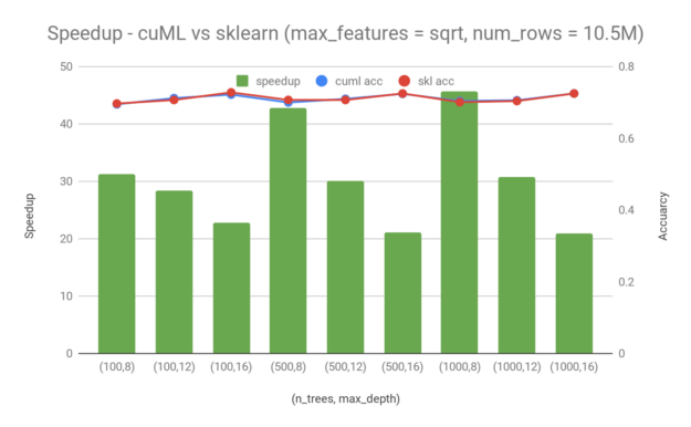
From these examples, you can see a 20x — 45x speedup by switching from sklearn to cuML for random forest training. Random forest in cuML is faster, especially when the maximum depth is lower and the number of trees is smaller. Moreover, in the case when there are 1000 trees and the maximum depth is 16, cuML still has a ~20x speedup compared to sklearn. It is worth mentioning that the speedup that you get from cuML comes without sacrificing accuracy. The accuracy difference between cuML and sklearn is minimal for the Higgs dataset.

We also repeated the experiments with the make_classification dataset available from sklearn. For a dataset of 1M samples and 100 features, we saw a speedup in the range of 25–60x. The difference in accuracy between sklearn and cuml is minimal here as well.

Bar chart — *Figure 4. Speedup of cuML vs. sklearn.*

Multi-GPU with Dask

To fully understand the best performance that you can get from random forest training using GPUs, we extended the test to multi-GPU runs using the Dask-based distributed approach mentioned earlier. Figure 4 showcases the speedup of multi-GPU runs compared to single-GPU. We used the same dataset (Higgs with 8.8M rows to train and 1000 rows to test) and the same hardware (DGX-1 server with eight V100–16-GB GPUs) in this section. For the multi-GPU tests, we chose to use 1000 trees per model and a maximum depth equal to 8, 12, or 16.

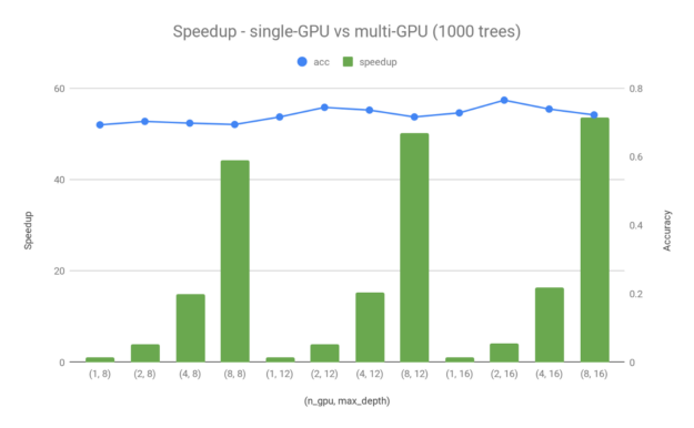
Figure 4 shows a ~40–50x speedup for max_depth=16 when using eight V100 GPUs instead of one. As discussed in the Example: Building forests across multiple GPUs section, both the dataset and trees are distributed across multiple GPUs. This is why you can get better than linear speedup scaling across multiple devices. There are indeed some small differences in terms of accuracy between single-GPU and multi-GPU runs, which is to be expected given the different data distributions. However, these small accuracy differences can almost be neglected with the large performance gain that you get by scaling the training to multiple devices.

Known limitations

For some applications (particularly large-scale regression problems), increasing n_bins may improve accuracy. In the current version, larger n_bins values can sometimes lead to significant slowdowns. The team is working on potential optimizations to reduce these slowdowns.

Accelerating Random Forests Up to 45x Using cuML