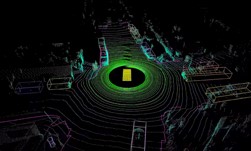
Many Jetson users choose lidars as their major sensors for localization and perception in autonomous solutions. Lidars describe the spatial environment around the vehicle as a collection of three-dimensional points known as a point cloud. Point clouds sample the surface of the surrounding objects in long range and high precision, which are well-suited for use in higher-level obstacle perception, mapping, localization, and planning algorithms.
Processing point clouds with CUDA-PCL
In this post, we introduce CUDA-PCL 1.0, which includes three CUDA-accelerated PCL libraries:
- CUDA-ICP
- CUDA-Segmentation
- CUDA-Filter
| NVIDIA Jetson | NVIDIA Xavier AGX 8GB |
| OS | Jetpack 4.4.1 |
| CUDA | 10.2 |
| PCL | 1.8 |
| Eigen | 3 |
CUDA-ICP
In the iterative closest point (ICP) one-point cloud—also known as an iterative corresponding point vertex cloud—the reference, or target, is kept fixed while the source is transformed to best match the reference. The algorithm iteratively revises the transformation needed to minimize an error metric, which is a combination of translation and rotation. This is usually a distance from the source to the reference point cloud, such as the sum of squared differences between the coordinates of the matched pairs. ICP is one of the widely used algorithms in aligning three-dimensional models, given an initial guess of the rigid transformation required.
The advantages of ICP are high accuracy-matching results, robust with different initialization, and so on. However, it consumes a lot of computing resources. To improve ICP performance on Jetson, NVIDIA released a CUDA-based ICP that can replace the original version of ICP in the Point Cloud Library (PCL).
Using CUDA-ICP
The following code example is the CUDA-ICP sample. You can instance the class and then implement cudaICP.icp() directly.
    cudaICP icpTest(nPCountM, nQCountM, stream);
    icpTest.icp(cloud_source, nPCount,
            float *cloud_target, int nQCount,
            int Maxiterate, double threshold,
            Eigen::Matrix4f &transformation_matrix, stream);
ICP calculates transformation_matrix between the two-point cloud:
source(P)* transformation =target(Q)
Because lidar provides the point cloud with the fixed number, you can get the maximum of points number. Both nPCountM and nQCountM are used to allocate cache for ICP.
class cudaICP
{
public:
    /*       nPCountM and nQCountM are the maximum of count for input clouds.
       They are used to pre-allocate memory.
    */
    cudaICP(int nPCountM, int nQCountM, cudaStream_t stream = 0);
    ~cudaICP(void);
    /*
    cloud_target = transformation_matrix *cloud_source
    When the Epsilon of the transformation_matrix is less than threshold,
    the function returns transformation_matrix.
    Input:
        cloud_source, cloud_target: Data pointer for the point cloud.
        nPCount: Point number of the cloud_source.
        nQCount: Point number of the cloud_target.
        Maxiterate: Threshold for iterations.
        threshold: When the Epsilon of the transformation_matrix is less than
            threshold, the function returns transformation_matrix.
    Output:
        transformation_matrix
    */
    void icp(float *cloud_source, int nPCount,
            float *cloud_target, int nQCount,
            int Maxiterate, double threshold,
            Eigen::Matrix4f &transformation_matrix,
            cudaStream_t stream = 0);
    void *m_handle = NULL;
};
| CUDA-ICP | PCl-ICP | |
| count of points cloud | 7000 | 7000 |
| maximum of iterations | 20 | 20 |
| cost time(ms) | 55.1 | 523.1 |
| fitness_score | 0.514 | 0.525 |
CUDA-Segmentation
A point cloud map contains many ground points. This not only makes the whole map look messy but also brings trouble to the classification, identification, and tracking of subsequent obstacle point clouds, so it needs to be removed first. Ground removal can be achieved by point cloud segmentation. The lib uses random sample consensus (Ransac) fitting and non-linear optimization to implement it.
Using CUDA-Segmentation
The following code example is the CUDA-Segmentation sample. Instance the class, initialize parameters, and then implement cudaSeg.segment directly.
  //Now Just support: SAC_RANSAC + SACMODEL_PLANE
  std::vector<int> indexV;
  cudaSegmentation cudaSeg(SACMODEL_PLANE, SAC_RANSAC, stream);
  segParam_t setP;
  setP.distanceThreshold = 0.01;
  setP.maxIterations = 50;
  setP.probability = 0.99;
  setP.optimizeCoefficients = true;
  cudaSeg.set(setP);
  cudaSeg.segment(input, nCount, index, modelCoefficients);
  for(int i = 0; i < nCount; i++)
  {
    if(index[i] == 1)
    indexV.push_back(i);
  }
CUDA-Segmentation segments input that has nCount points with parameters. index is the index of input that is the target plane and modelCoefficients is the group of coefficients of the plane.
typedef struct {
  double distanceThreshold;
  int maxIterations;
  double probability;
  bool optimizeCoefficients;
} segParam_t;
class cudaSegmentation
{
public:
    //Now Just support: SAC_RANSAC + SACMODEL_PLANE
    cudaSegmentation(int ModelType, int MethodType, cudaStream_t stream = 0);
    ~cudaSegmentation(void);
    /*
    Input:
        cloud_in: Data pointer for point cloud
        nCount: Count of points in cloud_in
    Output:
        Index: Data pointer that has the index of points in a plane from input
      modelCoefficients: Data pointer that has the group of coefficients of the plane
    */
    int set(segParam_t param);
    void segment(float *cloud_in, int nCount,
            int *index, float *modelCoefficients);
private:
    void *m_handle = NULL;
};
| CUDA-Segmentation | PCL-Segmentation | |
| count of points cloud | 11w+ | 11w+ |
| Points selected | 7519 | 7519 |
| cost time(ms) | 55.1 | 364.2 |
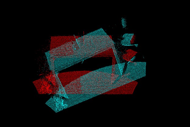
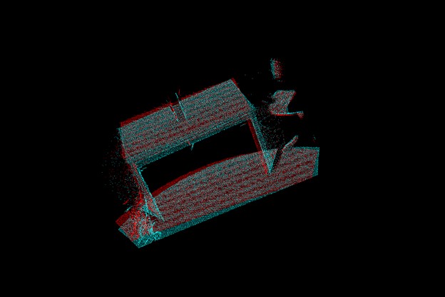
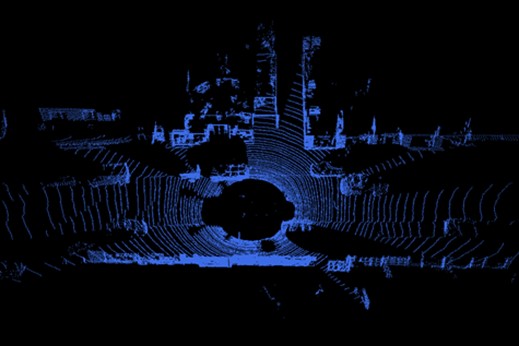
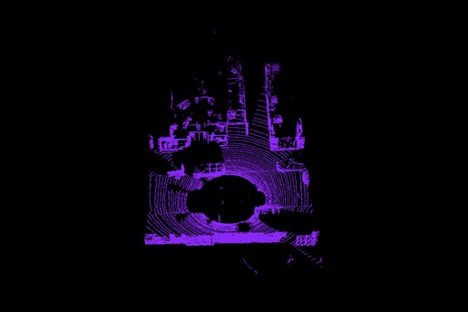
Figures 3 and 4 show the original point cloud data and then a version processed with only obstacle-related point clouds remaining. This example is typical in point cloud processing, including ground removal, removing some point clouds, and feature extraction, clustering some point clouds.

CUDA-Filter
Filtering is one of the most important preprocessing operations for point clouds before segmentation, detection, recognition, and so on. The PassThrough filter is the simplest, roughest method, which filters the point cloud coordinate constraints on the X, Y, and Z axes of the point clouds directly. Point cloud filtering can be achieved by constraint only on the Z axis or the three coordinate axes X, Y, and Z. CUDA-Filter currently supports only PassThrough, but will support more methods later.
Using CUDA-Filter
The following code example is the CUDA-Filter sample. Instance the class, initialize parameters, and then implement cudaFilter .filter directly.
  cudaFilter filterTest(stream);
  FilterParam_t setP;
  FilterType_t type = PASSTHROUGH;
  setP.type = type;
  setP.dim = 2;
  setP.upFilterLimits = 1.0;
  setP.downFilterLimits = 0.0;
  setP.limitsNegative = false;
  filterTest.set(setP);
  filterTest.filter(output, &countLeft, input, nCount);
CUDA-Filter filters input that has nCount points with parameters and output has countLeft points filtered by CUDA.
typedef struct {
    FilterType_t type;
    //0=x,1=y,2=z
    int dim;
    float upFilterLimits;
    float downFilterLimits;
    bool limitsNegative;
} FilterParam_t;
class cudaFilter
{
public:
    cudaFilter(cudaStream_t stream = 0);
    ~cudaFilter(void);
    int set(FilterParam_t param);
    /*
    Input:
        source: data pointer for point cloud
        nCount: count of points in cloud_in
    Output:
        output: data pointer which has points filtered by CUDA
        countLeft: count of points in output
    */
    int filter(void *output, unsigned int *countLeft, void *source, unsigned int nCount);
    void *m_handle = NULL;
};
| CUDA-Filter | PCL-Filter | |
| count of points cloud | 11w+ | 11w+ |
| dim | Z | Z |
| down,up FilterLimits | (0.0,1.0) | (0.0,1.0) |
| limitsNegative | false | false |
| Points selected | 15860 | 15860 |
| cost time(ms) | 0.589752 | 2.82811 |
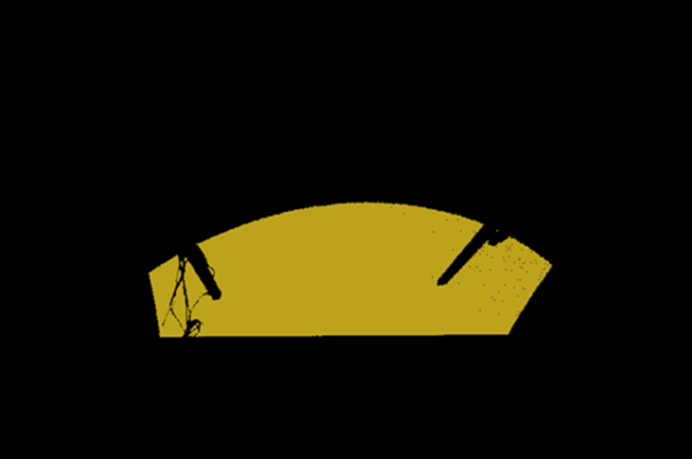
Figures 5 and 6 shows an example of the PassThrough filter by constraint on the X axis.
Get started with CUDA-PCL
In this post, we showed you how to use CUDA-PCL to get the best performance. Because PCL cannot take advantage of CUDA from Jetson, we developed some libraries that have the same functions with PCL but which are based on CUDA. Download the libraries and demo.
