Loading data onto GPUs for training has historically been a minor issue for most deep learning practitioners. Data read from a local spinning hard drive or NAS device would be preprocessed on the CPU, then shipped to the GPU for training. The data input pipeline rarely proved to be the bottleneck given the long number-crunching times involved.
As GPUs improve and DL frameworks use them more efficiently, however, it becomes increasingly harder to feed the GPU with data fast enough to keep up with training. Framework developers have to optimize input pipelines and use many CPU cores per GPU to preprocess the data. The random access pattern of training means that training data must now be stored on an SSD, or even an array of SSDs, instead of spinning disks, significantly increasing the cost of deep learning systems.
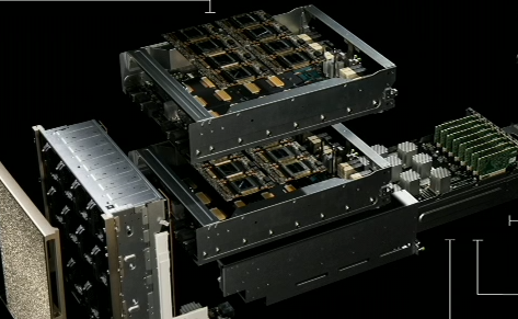
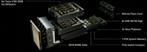
Data input pipelines will only become a greater bottleneck with advances like the TensorCores in the latest GPUs and NVSwitch, which allows more GPUs in each server. Increasing dataset sizes and the increasing importance of video as a data source means the amount of high-performance SSD storage local to the training server continues to grow, becoming a larger portion of the overall cost of the server. Figure 1 shows NVIDIA’s DGX-2 high-performance compute engine, which incorporates NVLink switches for high data throughput.
In this post, we show how you can eliminate the data input bottleneck and reduce the local storage requirements when training on video data by utilizing the video decompression hardware in NVIDIA GPUs in your input pipeline. The NVIDIA Video Loader (NVVL), an open source library that we recently released, handles all the heavy lifting for you. Using NVVL requires minimal changes to your existing code base to realize a significant improvement.
Why Bother with Acceleration?
The relative amount of disk storage and throughput, CPU processing, and PCIe bandwidth in a system has been falling substantially compared to the amount of available GPU processing. This is especially true when training on video datasets. These datasets quickly become very large and unwieldy, requiring large numbers of expensive SSDs and multiple CPU cores to read and prepare the data fast enough for the GPU training process to use.
All modern NVIDIA GPUs have hardware dedicated to decompressing video. Using this hardware allows us to store highly-compressed data using modern video codecs such as H.264 and HEVC, only decompressing it just in time for training on the GPU. This dramatically reduces the amount of high-performance storage needed in DL training systems. Since the GPU decompresses the video, this makes it convenient to use the GPU for any preprocessing, such as cropping and resizing, that must be done before training. This enables a larger ratio of GPUs per CPU core in the system. Reducing the amount of high-performance storage and CPUs required to keep the GPUs training at full speed dramatically simplifies system design and reduces the cost of deep learning systems.
We trained the video super-resolution network described in End-to-End Learning of Video Super-Resolution with Motion Compensation [Makansi 2017] using PyTorch to quantify the advantages of accelerating a video input pipeline. We first look at space saved using video files directly versus storing individual frames as image files. We prepare the Myanmar videos available from Harmonic, Inc [Harmonic 2014] for training as described below using FFmpeg and libx264 and libx265. We compare each frame to a losslessly compressed downsample of the original source video stored as PNG files. We also performed the same comparison using frames stored as compressed JPEGs using FFmpeg’s mjpeg encoder. We use the arithmetic mean of the peak signal-to-noise ratio (PSNR) across all frames in the training and validation set to estimate the quality of the frames. You can see the results in figure 2.
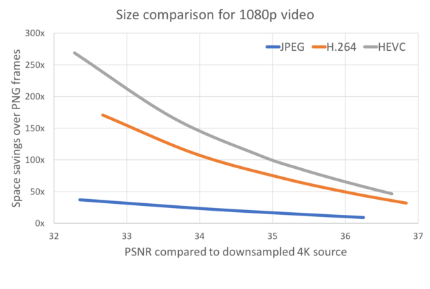
As you can see, storing the training data as videos provides enormous space savings over storing the data as individual PNG files and significant savings over storing the data as individual JPEG files. The actual amount of space savings depends heavily on the quality needed for the application. As the quality needed increases the amount of space saved decreases.
At a high quality of 36 PSNR (in this case achieved with a CRF of 18), an H.264 file is 47x smaller than the PNG files while HEVC is 70x smaller. If such high-quality frames are not necessary, the savings can get much larger: an HEVC file with a PSNR of 32.3 is 269x smaller than PNG files. On average, JPEG files of similar quality are 7.5x larger than an HEVC file and 5x an H.264 file. Depending on the application, it may possible to do a significant amount of training using highly compressed frames then fine-tune the model using a smaller dataset of high-quality video.
We measured the mini-batch data loading overhead, host CPU consumption, and host memory consumption for NVVL as compared to three other data loaders implemented in PyTorch. This helped us assess the speed and resource consumption benefits of NVVL in deep learning training scenarios. We implemented a data loader for H.264 encoded videos in mp4 containers using NVVL, a second data loader for videos using ffmpeg for decoding using the recently released Lintel library [Duke 2018], and data loaders for JPEG and PNG files following standard PyTorch examples. We carried out comparisons for a range of source data resolutions (540p, 720p, 1080p, 4K) cropped to 540p to represent a reasonable input to a modern neural network. We also carried out all experiments with the final neural network input data in both FP32 and FP16. A complete table of these experimental results can be found and the code used for benchmarking is here.
Let’s look at the data loading performance for FP32 PyTorch tensors to a single V100 GPU in mini-batches of 8 samples. These results are representative of what we see for FP32 and multi-GPU loading. Data loading overhead quantifies how much additional time is added by each data loader to each training iteration, i.e. data loading computation and data transfer that cannot be carried out asynchronously with neural network training computation. First, let’s look at data loading overhead, shown in figure 3.
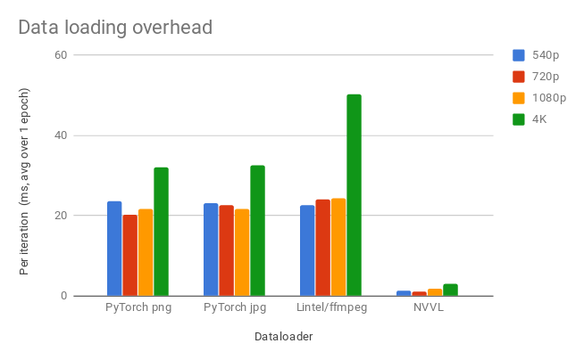
In Figure 3, we see that NVVL has significantly lower overhead across all resolutions and that overhead increases with resolution more slowly than for the other loaders.
Next, we look at CPU load – this is the average number of processes running across the CPUs in the host system at any given time over one training epoch.
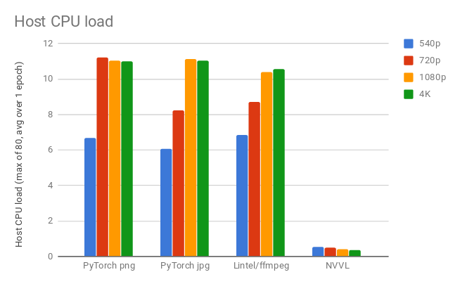
In Figure 4, we see that NVVL has significantly lower CPU load than all other loaders.
Finally, we look at instantaneous host memory usage averaged over one training epoch.
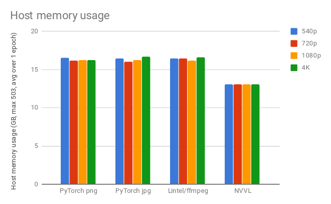
Once more we see in Figure 5 that NVVL has a lower resource demand, this time for host memory.
We also replicated the network described in End-to-End Learning of Video Super-Resolution with Motion Compensation [Makansi 2017] in order to demonstrate the use of NVVL in a realistic deep learning training application. We chose to train this network because it takes random frame sequences extracted from a collection of videos as input and requires no additional data labels. This enables scaling the training of this network to an almost unlimited amount of video data.
We trained the super-resolution network on the 8 GPUs of a V100 DGX-1 with 540p source data and batch size 7 using both NVVL and the PyTorch PNG data loader. Per iteration overhead introduced by the two loaders, seen in Figure 3, proved considerably smaller than the time spent in computation for this network. The resulting overhead effect was negligible and the two methods resulted in very similar training times. We also discovered that NVVL incurred 40% less CPU load and used 36% less host memory on top of the disk space savings.
Using NVVL
Preparing the data
NVVL supports the H.264 and HEVC (H.265) video codecs in any container format that FFmpeg is able to parse. Video codecs only store certain frames, called keyframes or intra-frames, as a complete image in the data stream. All other frames require data from other frames, either before or after it in time, to be decoded.
In order to decode a sequence of frames, decoding must start at the keyframe before the sequence and continue past the sequence to the next keyframe after it. This isn’t a problem when sequentially reading a video. However, when decoding small sequences of frames randomly throughout the video, a large gap between keyframes results in reading and decoding a large number of frames that are never used.
Videos used during training should be encoded with a relatively small keyframe interval to alleviate this problem. We’ve found setting the keyframe interval to the length of the sequences you will be reading provides a good compromise between file size and loading performance. For example, if you typically load 5 sequential frames at a time use a keyframe interval of 5. See the documentation for more information and flags to use when transcoding videos using FFmpeg.
Loading the data
NVVL has C and C++ APIs, but most users will want to use the provided PyTorch interface. Using NVVL in PyTorch is similar to using the standard PyTorch dataset and dataloader. We first create an nvvl.VideoDataset object to describe the data set. You must provide a list of filenames which must be video files such as mp4 or mkv files. You also need to supply the sequence length, which is the number of frames in each sample.
import nvvl
filenames = [“data01.mkv”, “data02.mkv”]
dataset = nvvl.VideoDataset(filenames, sequence_length=5)
The sequence length is the number of contiguous frames that each data item should be. Each element in the dataset corresponds to a sequence of frames beginning at a specific frame within a specific video file. You can optionally set the datatype that should be used (either “byte”, “half”, or “float”), the color space (RGB or YCrCb), and preprocessing (normalizing, scaling, cropping, and flipping) that should be done to each element. See the documentation for details.
This dataset object behaves similarly to a normal torch.utils.data.Dataset. You can access individual elements, get its length, and more. Retrieving individual elements from the dataset will synchronously transfer the encoded data to the GPU, decode it, then transfer the uncompressed data back to the CPU. Thus, elemental access of the dataset should not be done in performance critical code.
Once you have an nvvl.VideoDataset object, you use it to create an nvvl.VideoLoader which behaves similarly to a torch.utils.data.DataLoader.
loader = nvvl.VideoLoader(dataset, batch_size=8, shuffle=True)
Using elemental access to pass the pass the nvvl.VideoDataset to a normal DataLoader technically works. However, using elemental access would not perform well as described above. The nvvl.VideoLoader pipelines the decoding of frames and provides an entire batch already on the GPU in a torch.cuda.Tensor (or a tensor of the requested type). Once an iterator over the loader is created, it must be run to completion before another iterator is created and before any elemental access to the dataset due to this pipelining. Otherwise, the loader can be used just like any other PyTorch DataLoader:
for i, input in enumerate(loader):
loss = model(Variable(input))
loss.backward()
…
Get Started with NVVL
You now have a taste of how easy it is to use NVVL in your PyTorch training code. Get started with NVVL by going to the github project . You’ll find documentation for the C and C++ interface to help you if you use a framework other than PyTorch and want to write your own wrapper for that framework. You’ll also find a more detailed run-through and further documentation of the PyTorch interface as a well as the full source code to our super resolution example used in the performance testing described above.
Acknowledgments
We would like to thank Brendan Duke, the author of Lintel, for helpful discussion about optimal utilization of his library.
Further Reading
“Storage Performance Basics for Deep Learning”
References
[Makansi 2017] End-to-End Learning of Video Super-Resolution with Motion Compensation arXiv:1707.00471, 2017
[Harmonic 2014] Myanmar 60p, Harmonic Inc. (2014), [online]. Available at https://www. harmonicinc.com/resources/videos/4k-video-clip-center
[Duke 2018] https://github.com/dukebw/lintel
