
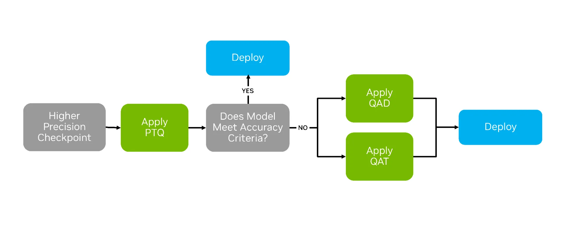
After training AI models, a variety of compression techniques can be used to optimize them for deployment. The most common is post-training quantization (PTQ), which applies numerical scaling techniques to approximate model weights in lower-precision data types. But two other strategies—quantization aware training (QAT) and quantization aware distillation (QAD)—can succeed where PTQ falls short by actively preparing the model for life in lower precision (See Figure 1 below).
QAT and QAD aim to simulate the impact of quantization during post-training, allowing higher-precision model weights and activations to adapt to the new format’s representable range. This adaptation provides a smoother transition from higher to lower precisions, often yielding greater accuracy recovery.
In this blog, we explore QAT and QAD, and demonstrate how to apply them with the TensorRT Model Optimizer. Model Optimizer provides APIs that are natively compatible with Hugging Face and PyTorch, enabling developers to seamlessly prepare models for QAT/QAD while leveraging familiar training workflows. Once the final model is trained using these techniques, we demonstrate how to efficiently export and deploy them with TensorRT-LLM.
What is Quantization Aware Training?
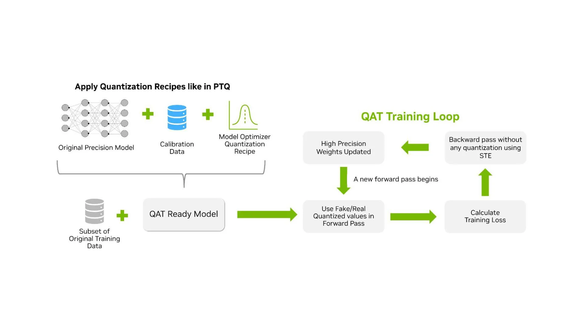
QAT is a technique in which the model learns to handle low-precision arithmetic during an additional training phase after pre-training. Unlike PTQ, which quantizes a model after full-precision training using a calibration dataset, QAT trains the model with quantized values in the forward path. The QAT workflow is nearly identical to the PTQ workflow; the key difference is that a training phase is injected after the quantization recipe has been applied to the original model (Figure 2 below).
The goal of QAT is to produce a quantized model with high accuracy for inference performance. This makes QAT different from quantized training, which targets improvements in training efficiency. QAT may therefore use methods that are not optimal for training throughput but result in a more accurate model for inference.
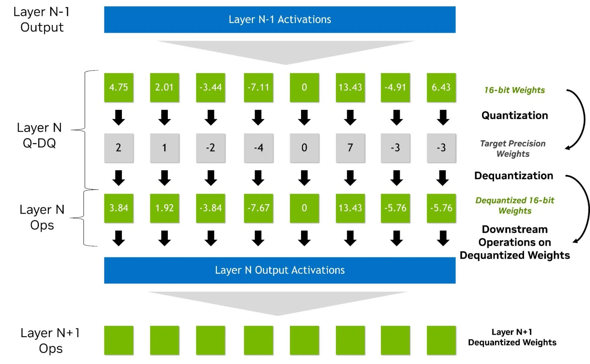
QAT is typically performed with “fake quantized” weights and activations in the forward pass. In this approach, lower precision is represented within a higher data type through a quantize/dequantize operator (See Figure 3 below). As a result, QAT does not require native hardware support. QAT for NVFP4, for instance, can be carried out on Hopper GPUs using simulated quantization. It integrates naturally into existing higher precision pipelines, with backward gradients computed in higher precision and quantization modeled as a pass-through operation (straight-through estimation, STE). Additional steps, such as zeroing outlier gradients, may also be applied, adding overhead beyond BF16 or FP16.
By exposing the loss function to rounding and clipping errors during training, QAT enables the model to adapt and recover from them. In practice, QAT may not maximize training performance, but it provides a stable and practical training process that yields a high accuracy quantized inference model.
Some implementations of QAT/QAD do not require fake quantization, but those methods are out of scope of this blog. In the current Model Optimizer implementation, the output of QAT is a new model in the original precision with updated weights along with critical metadata for converting to the target format such as:
- Scaling factors (dynamic ranges) for each layer activation
- Quantization parameters such as bits
- Block size
How to apply QAT with Model Optimizer
Applying QAT with Model Optimizer is fairly straightforward. QAT supports the same quantization formats as the PTQ workflow, including key formats such as FP8, NVFP4, MXFP4, INT8, and INT4. For the code snippet below, we selected NVFP4 weight and activation quantization.
import modelopt.torch.quantization as mtq

config = mtq.NVFP4_MLP_ONLY_CFG

# Define forward loop for calibration
def forward_loop(model):
    for data in calib_set:
        model(data)

# quantize the model and prepare for QAT
model = mtq.quantize(model, config, forward_loop)
Up to this point, the code is identical to PTQ. To apply QAT, we need to perform a training loop. This loop includes standard tunable parameters such as the choice of optimizer, scheduler, learning rate, and so on.
# QAT with a regular finetuning pipeline
# Adjust learning rate and training epochs
train(model, train_loader, optimizer, scheduler, ...)
For optimal results, we suggest running QAT for a duration equivalent to about 10% of the initial training epochs. In the context of LLMs, we’ve observed that QAT fine-tuning for even less than 1% of the original pre-training time is often sufficient to restore the model’s quality. To dive deeper into QAT, we recommend exploring the complete Jupyter notebook walkthrough.
What is Quantization Aware Distillation?
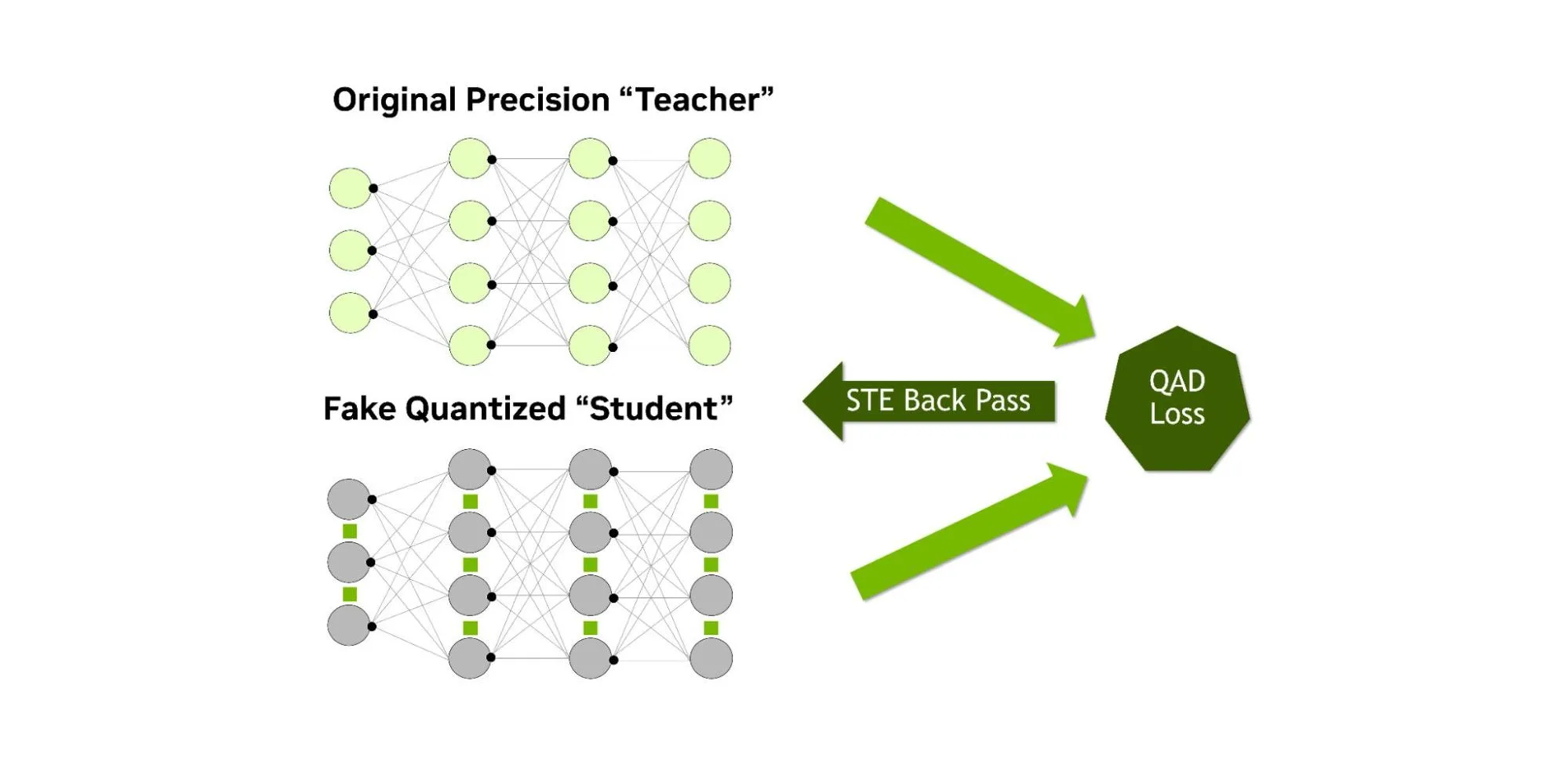
Similar to QAT, QAD aims to recover accuracy after post-training quantization, but it simultaneously performs knowledge distillation. Unlike standard knowledge distillation, where a larger “teacher” model guides a smaller “student” model, the student in QAD is simply leveraging fake quantization during the forward pass. The teacher model is the original higher precision model that has already been trained on the same data. The distillation process aligns the quantized student’s outputs with the full-precision teacher’s outputs, using a distillation loss to measure how far the quantized predictions deviate (Figure 4 below).
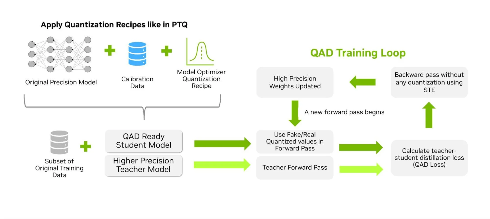
The student’s computations are fake quantized during the distillation process while the teacher remains at full precision. Any mismatch introduced by quantization is directly exposed to the distillation loss, allowing the low-precision weights and activations to adjust toward the teacher’s behavior (Figure 5 below). After QAD, the resulting model runs with the same inference performance as PTQ and QAT (since precision and the architecture are unchanged), but the accuracy recovery can be higher, thanks to the additional learning provided by the distillation loss.
In practice, this approach is more effective than distilling a FP32 model and then quantizing it, since the QAD process is better able to take into account the quantization error and adjust the model directly to account for it.
How to apply QAD with Model Optimizer
TensorRT Model Optimizer currently provides experimental APIs for applying this technique. Starting with a process similar to QAT and PTQ, the quantization recipe must first be applied to the student model. After that, the distillation configuration can be defined, specifying elements such as the teacher model, training arguments, and the distillation loss function. The QAD APIs will undergo improvements to simplify the application of this technique. To track the latest code examples and documentation, explore the QAD section of the Model Optimizer repository.
Evaluating the Impact of QAT and QAD
Not all models require QAT or QAD—many retain over 99.5% of their original accuracy across key benchmarks with just PTQ.
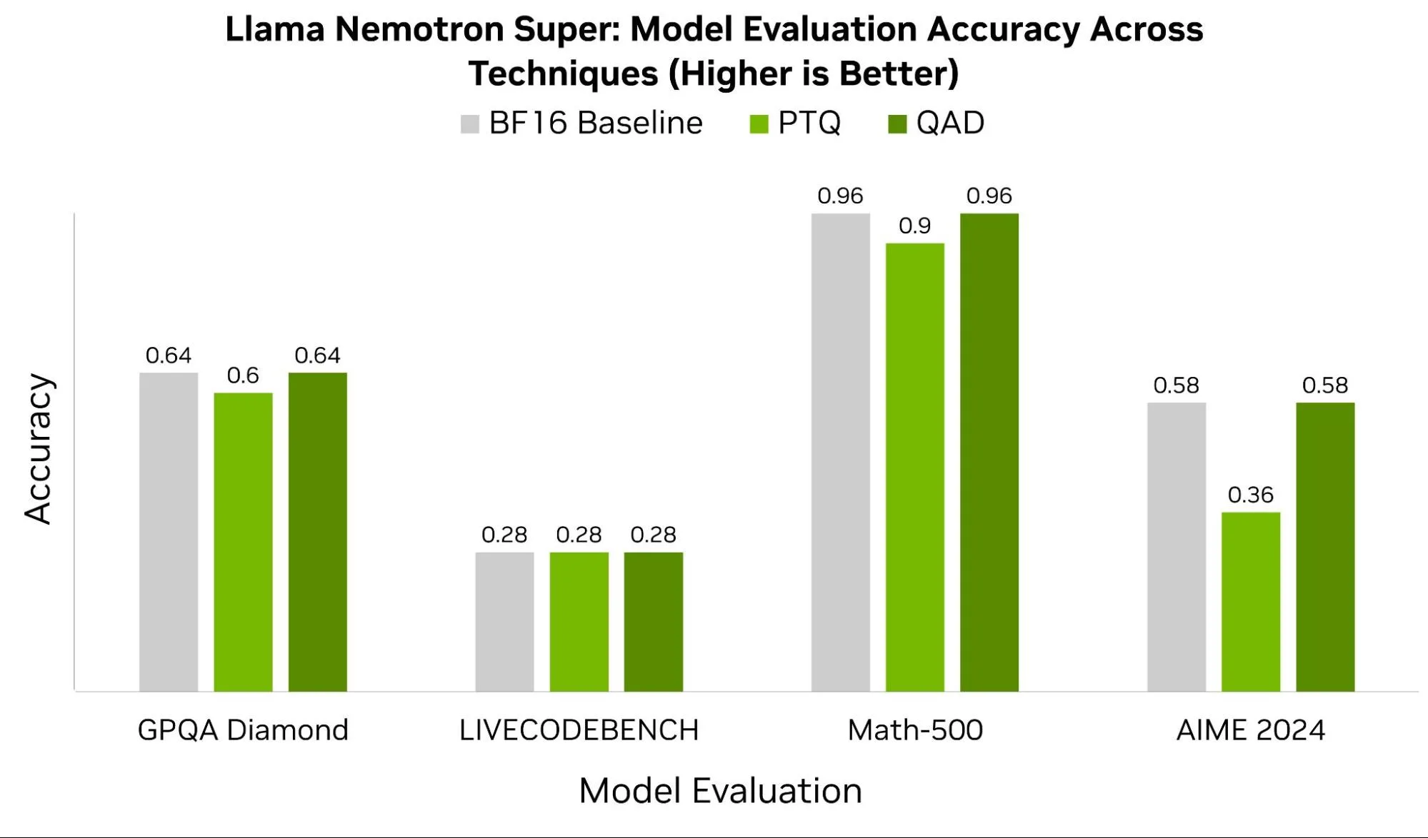
In some cases, like that of Llama Nemotron Super, we observe significant benefits from QAD. Figure 6 below compares this model’s baseline BF16 scores across benchmarks such as GPQA Diamond, LIVECODEBENCH, Math-500, and AIME 2024 to the checkpoints after PTQ and QAD. With the exception of LIVECODEBENCH, all other benchmarks recover at least 4-22% accuracy leveraging QAD.
In practice, the success of QAT and QAD depends heavily on the quality of the training data, the chosen hyperparameters, and the model architecture. When quantizing down to 4-bit data types, formats like NVFP4 benefit from more granular and higher-precision scaling factors.
Figure 7 below shows accuracy for Llama-Nemotron Nano across common VLM benchmarks for both NVFP4 and MXFP4. Across benchmarks like AI2D, ChartQA, and DocVQA, we see NVFP4 consistently scoring higher by less than 1%. Though small, these small differences can lead to observable impact in real-world tasks. On the OpenVLM Hugging Face Leaderboard, the performance gap between the top model and lower-ranked models on a given benchmark is often just a few points.
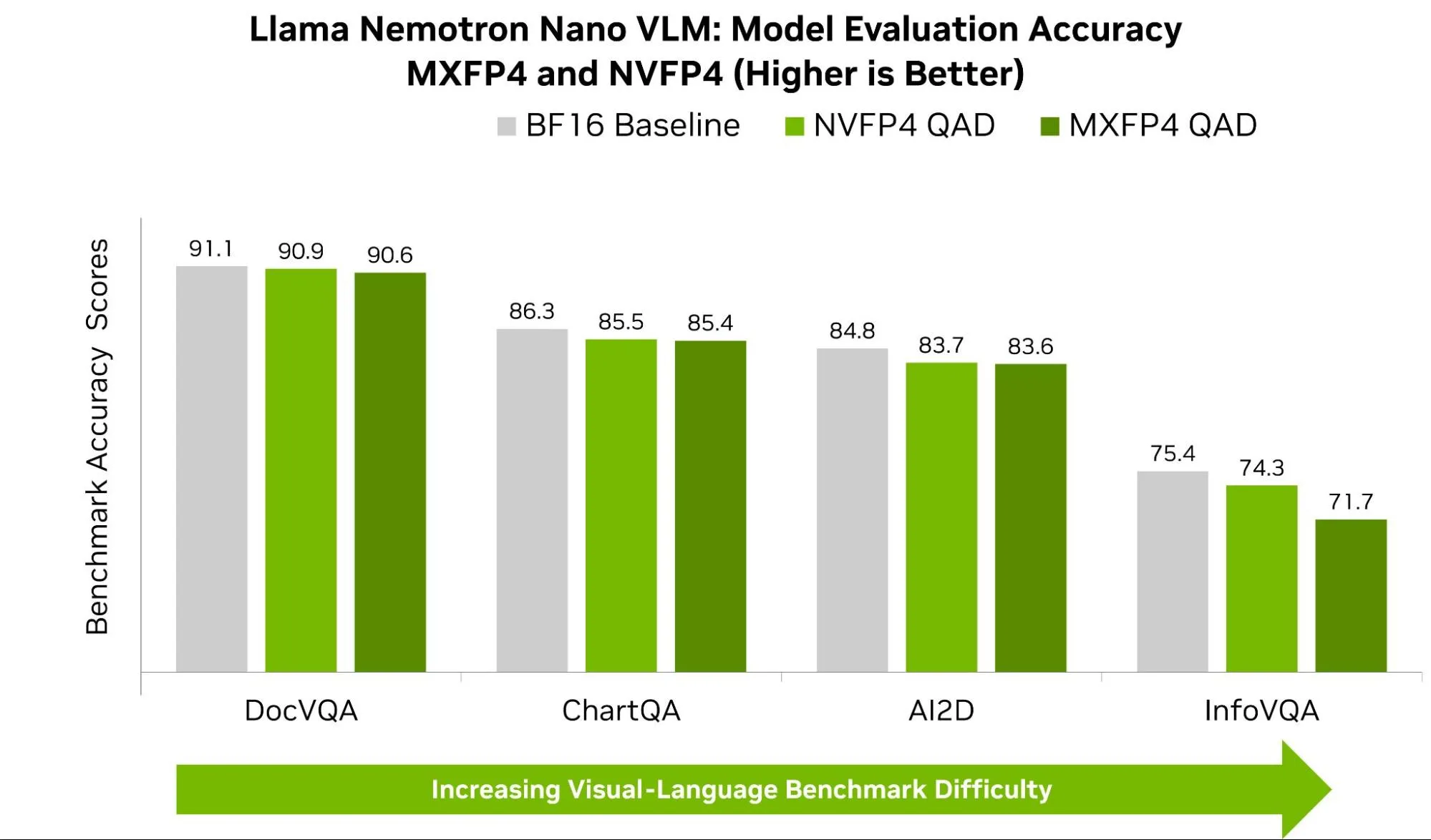
A larger gap is observed between visual question answering (VQA) like InfoVQA and DocVQA. InfoVQA and DocVQA both ask questions about images, but they stress different things during inference. InfoVQA’s dataset is composed of busy charts and complex graphics with tiny numbers, thin lines, and nuanced annotations. When the model is quantized to 4 bits, we risk rounding away the model’s ability to detect those small details. NVFP4 helps here because it uses finer-grained scaling (smaller blocks and higher-precision scale factors), which better preserves both small signals and occasional outliers—yielding steadier alignment between the visual and text components of the model (less rounding/clipping error).
DocVQA, by contrast, is mostly clean, structured documents (forms, invoices, receipts) where once the right field is found, the answer is obvious—so both formats are already near the ceiling, and the gap stays small.
Summary
Quantization aware training (QAT) and quantization aware distillation (QAD) extend the benefits of PTQ by teaching models to adapt directly to low-precision environments, recovering accuracy where simple calibration falls short. As shown in benchmarks like Math-500 and AIME 2024, these techniques can close the gap between low-precision inference and full-precision baselines, giving developers the best of both worlds: the efficiency of FP4 execution and the robustness of high-precision training. Considerations must be made for dataset selection and training hyperparameters as these can have a significant impact on the result of this technique.
With TensorRT Model Optimizer, these advanced workflows are accessible through familiar PyTorch and Hugging Face APIs, making it easy to experiment with formats such as NVFP4 and MXFP4. Whether you need the speed of PTQ, the resilience of QAT, or the accuracy gains of QAD, you have a complete toolkit to compress, fine-tune, and deploy models on NVIDIA GPUs. The result is faster, smaller, and more accurate AI—ready for production at scale.
To explore further, check-out our Jupyter notebook tutorials.
