在 xgboost1 . 0 中,我们引入了 新的官方 Dask 接口 来支持高效的分布式训练。 快速转发到 XGBoost1 . 4 ,接口现在功能齐全。如果您对 xgboostdask 接口还不熟悉,请参阅第一篇文章,以获得一个温和的介绍。在本文中,我们将看一些简单的代码示例,展示如何最大化 GPU 加速的好处。
我们的例子集中在希格斯数据集上,这是一个来自 机器学习库 的中等规模的分类问题。 在下面的章节中,我们从基本数据加载和预处理开始,使用 GPU 加速的 Dask 和 Dask-ml 。然后,针对不同配置的返回数据训练 XGBoost 模型。同时,分享一些新特性。之后,我们将展示如何在 GPU 集群上计算 SHAP 值以及可以获得的加速比。最后,我们分享了一些优化技术与推理。
以下示例需要在至少有一个 NVIDIA GPU 的机器上运行, GPU 可以是笔记本电脑或云实例。 Dask 的优点之一是它的灵活性,用户可以在笔记本电脑上测试他们的代码。它们还可以将计算扩展到具有最小代码更改量的集群。 另外,要设置环境,我们需要 xgboost==1.4 、 dask 、 dask-ml 、 dask-cuda 和 达斯克 – cuDF python 包,可从 RAPIDS 康达频道: 获得
conda install -c rapidsai -c conda-forge dask dask-ml dask-cuda dask-cudf xgboost=1.4.2在 GPU 集群上用 Dask 加载数据
首先,我们将数据集下载到 data 目录中。
mkdir data
curl http://archive.ics.uci.edu/ml/machine-learning-databases/00280/HIGGS.csv.gz --output ./data/HIGGS.csv.gz
然后使用 dask-cuda 设置 GPU 集群:
import os
from time import time
from typing import Tuple

from dask import dataframe as dd
from dask_cuda import LocalCUDACluster
from distributed import Client, wait
import dask_cudf
from dask_ml.model_selection import train_test_split

import xgboost as xgb
from xgboost import dask as dxgb
import numpy as np
import argparse

# … main content to be inserted here in the following sections

if __name__ == "__main__":
   parser = argparse.ArgumentParser()
   parser.add_argument("--n_workers", type=int, required=True)
   args = parser.parse_args()
   with LocalCUDACluster(args.n_workers) as cluster:
       print("dashboard:", cluster.dashboard_link)
       with Client(cluster) as client:
           main(client)
给定一个集群,我们开始将数据加载到 gpu 中。 由于在参数调整期间多次加载数据,因此我们将 CSV 文件转换为 Parquet 格式以获得更好的性能。 这可以使用 dask_cudf 轻松完成:
def to_parquet() -> str:
   """Convert the HIGGS.csv file to parquet files."""
   dirpath = "./data"
   parquet_path = os.path.join(dirpath, "HIGGS.parquet")
   if os.path.exists(parquet_path):
       return parquet_path
   csv_path = os.path.join(dirpath, "HIGGS.csv")
   colnames = ["label"] + ["feature-%02d" % i for i in range(1, 29)]
   df = dask_cudf.read_csv(csv_path, header=None, names=colnames, dtype=np.float32)
   df.to_parquet(parquet_path)
   return parquet_path
数据加载后,我们准备培训/验证拆分:
def load_higgs(
    path,
) -> Tuple[
    dask_cudf.DataFrame, dask_cudf.Series, dask_cudf.DataFrame, dask_cudf.Series
]:
    df = dask_cudf.read_parquet(path)

    y = df["label"]
    X = df[df.columns.difference(["label"])]

    X_train, X_valid, y_train, y_valid = train_test_split(
        X, y, test_size=0.33, random_state=42
    )
    X_train, X_valid, y_train, y_valid = client.persist(
        [X_train, X_valid, y_train, y_valid]
    )
    wait([X_train, X_valid, y_train, y_valid])

    return X_train, X_valid, y_train, y_valid
在前面的示例中,我们使用 dask-cudf 从磁盘加载数据,使用 dask-ml 中的 火车测试分裂了 函数拆分数据集。 大多数时候, dask 的 GPU 后端与 dask-ml 中的实用程序无缝地工作,我们可以加速整个 ML 管道。
提前停止训练
最常请求的特性之一是提前停止对 Dask 接口的支持。 在 XGBoost1 . 4 版本中,我们不仅可以指定停止轮的数量,还可以开发定制的提前停止策略。 对于最简单的情况,向 train 函数提供停止回合可以实现提前停止:
def fit_model_es(client, X, y, X_valid, y_valid) -> xgb.Booster:
   early_stopping_rounds = 5
   Xy = dxgb.DaskDeviceQuantileDMatrix(client, X, y)
   Xy_valid = dxgb.DaskDMatrix(client, X_valid, y_valid)
   # train the model
   booster = dxgb.train(
       client,
       {
           "objective": "binary:logistic",
           "eval_metric": "error",
           "tree_method": "gpu_hist",
       },
       Xy,
       evals=[(Xy_valid, "Valid")],
       num_boost_round=1000,
       early_stopping_rounds=early_stopping_rounds,
   )["booster"]
   return booster
在前面的片段中有两件事需要注意。 首先,我们指定触发提前停止训练的轮数。 XGBoost 将在连续 X 轮验证指标未能改善时停止培训过程,其中 X 是指定提前停止的轮数。 其次,我们使用名为 DaskDeviceQuantileDMatrix 的数据类型进行训练,但使用 DaskDMatrix 进行验证。 DaskDeviceQuantileDMatrix 是 DaskDMatrix 的替代品,用于基于 GPU 的训练输入,避免了额外的数据拷贝。
与 gpu_hist 一起使用时, DaskDeviceQuantileDMatrix 可以节省大量内存,并且输入数据已经在 GPU 上。图 1 描述了 DaskDeviceQuantileDMatrix. 的结构 数据分区不再需要复制和连接,取而代之的是,由草图算法生成的摘要被用作真实数据的代理。
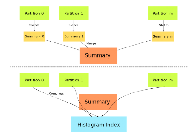
图 1 : DaskDeviceQuantileDMatrix 的构造 .
在 XGBoost 中,提前停止作为回调函数实现。 新的回调接口可以用来实现更高级的提前停止策略。下面的代码显示了提前停止的另一种实现,其中有一个附加参数要求 XGBoost 仅返回最佳模型,而不是完整模型:
  def fit_model_customized_es(client, X, y, X_valid, y_valid):
    early_stopping_rounds = 5
    es = xgb.callback.EarlyStopping(rounds=early_stopping_rounds, save_best=True)
    Xy = dxgb.DaskDeviceQuantileDMatrix(client, X, y)
    Xy_valid = dxgb.DaskDMatrix(client, X_valid, y_valid)
    # train the model
    booster = xgb.dask.train(
        client,
        {
            "objective": "binary:logistic",
            "eval_metric": "error",
            "tree_method": "gpu_hist",
        },
        Xy,
        evals=[(Xy_valid, "Valid")],
        num_boost_round=1000,
        callbacks=[es],
    )["booster"]
    return booster
在前面的示例中, EarlyStopping 回调作为参数提供给 train ,而不是使用 early_stopping_rounds 参数。为了提供一个定制的提前停止策略,探索 EarlyStopping 的其他参数或子类化这个回调是一个很好的起点。
定制目标和评估指标
XGBoost 被设计成可以通过定制的目标函数和度量进行扩展。在 1 . 4 中,这个特性被引入 dask 接口。要求与单节点接口完全相同:
def fit_model_customized_objective(client, X, y, X_valid, y_valid) -> dxgb.Booster:
    def logit(predt: np.ndarray, Xy: xgb.DMatrix) -> Tuple[np.ndarray, np.ndarray]:
        predt = 1.0 / (1.0 + np.exp(-predt))
        labels = Xy.get_label()
        grad = predt - labels
        hess = predt * (1.0 - predt)
        return grad, hess

    def error(predt: np.ndarray, Xy: xgb.DMatrix) -> Tuple[str, float]:
        label = Xy.get_label()
        r = np.zeros(predt.shape)
        predt = 1.0 / (1.0 + np.exp(-predt))
        gt = predt > 0.5
        r[gt] = 1 - label[gt]
        le = predt <= 0.5
        r[le] = label[le]
        return "CustomErr", float(np.average(r))

    # Use early stopping with custom objective and metric.
    early_stopping_rounds = 5
    # Specify the metric we want to use for early stopping.
    es = xgb.callback.EarlyStopping(
    rounds=early_stopping_rounds, save_best=True, metric_name="CustomErr"
    )

    Xy = dxgb.DaskDeviceQuantileDMatrix(client, X, y)
    Xy_valid = dxgb.DaskDMatrix(client, X_valid, y_valid)
    booster = dxgb.train(
        client,
        {"eval_metric": "error", "tree_method": "gpu_hist"},
        Xy,
        evals=[(Xy_valid, "Valid")],
        num_boost_round=1000,
        obj=logit,  # pass the custom objective
        feval=error,  # pass the custom metric
        callbacks=[es],
    )["booster"]
    return booster
在前面的函数中,我们使用定制的目标函数和度量来实现一个 logistic 回归模型以及提前停止。请注意,该函数同时返回 gradient 和 hessian , XGBoost 使用它们来优化模型。 另外,需要在回调中指定名为 metric_name 的参数。它用于通知 XGBoost 应该使用自定义错误函数来评估早期停止标准。
解释模型
在得到我们的第一个模型之后,我们 MIG ht 想用 SHAP 来解释预测。 SHapley 加法解释( SHapley Additive explainstructions , SHapley Additive explainstructions )是一种基于 SHapley 值解释机器学习模型输出的博弈论方法。 有关算法的详细信息,请参阅 papers 。 由于 XGBoost 现在支持 GPU 加速的 Shapley 值,因此我们将此功能扩展到 Dask 接口。现在,用户可以在分布式 GPU 集群上计算 shap 值。这是由显著改进的预测函数和 GPUTreeShap 库 实现的:
def explain(client, model, X):
   # Use array instead of dataframe in case of output dim is greater than 2.
   X_array = X.values
   contribs = dxgb.predict(
       client, model, X_array, pred_contribs=True, validate_features=False
   )
   # Use the result for further analysis
   return contribs
XGBoost 使用多个 GPU 计算 shap 值的性能如图 2 所示。
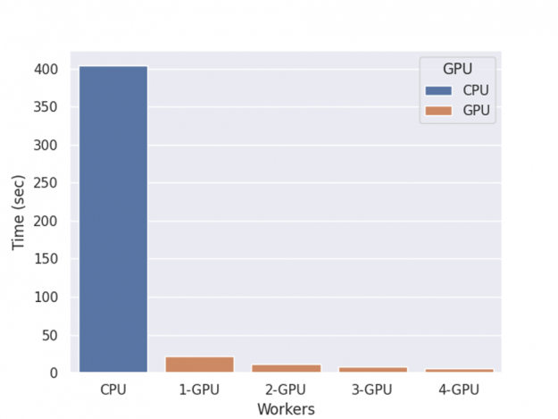
图 2 : Shap 推断时间。
基准测试是在一台 NVIDIA DGX-1 服务器上进行的,该服务器有 8 个 V100 gpu 和两个 20 核的 Xeon E5-2698 v4 cpu ,并进行了一轮训练、 shap 值计算和推理。
得到的 SHAP 值可用于可视化、使用特征权重调整列采样或用于其他数据工程目的。
运行推理
经过一些调整,我们得到了对新数据进行推理的最终模型。 XGBoost Dask 接口的预测没有旧版本那么有效,而且内存不足。在 1 . 4 中,我们修改了预测函数并增加了对就地预测的支持。 对于正态预测,它使用与 shap 值计算相同的接口:
def predict(client, model, X):
    predt = dxgb.predict(client, model, X)
    assert isinstance(predt, dd.Series)
    return predt
标准的 predict 函数提供了一个通用接口,可同时接受 DaskDMatrix 和 dask 集合(数据帧或数组),但没有针对内存使用进行优化。在这里,我们将其替换为就地预测,它支持基本的推理任务,并且不需要将数据复制到 XGBoost 的内部数据结构中:
def inplace_predict(client, model, X):
    # Use inplace_predict instead of standard predict.
    predt = dxgb.inplace_predict(client, model, X)
    assert isinstance(predt, dd.Series)
    return predt
内存节省取决于每个块的大小和输入类型。当使用同一模型多次运行推理时,另一个潜在的优化是对模型进行预格式化。默认情况下,每次调用 predict 时, XGBoost 都会将模型传输给 worker ,从而产生大量开销。好消息是 Dask 函数接受 future 对象作为完成模型的代理。然后我们可以传输数据,这些数据可以与其他计算和持久化数据重叠。
 def inplace_predict_multi_parts(client, model, X_train, X_valid):
    """Simulate the scenario that we need to run prediction on multiple datasets using train
	and valid. In real world the number of datasets is unlimited

    """
    # prescatter the model onto workers
    model_f = client.scatter(model)
    predictions = []
    for X in [X_train, X_valid]:
        # Use inplace_predict instead of standard predict.
        predt = dxgb.inplace_predict(client, model_f, X)
        assert isinstance(predt, dd.Series)
        predictions.append(predt)
        return predictions
在前面的代码片段中,我们将未来的模型传递给 XGBoost ,而不是真正的模型。 这样我们就避免了在预测过程中的重复传输,或者我们可以将模型传输与其他操作(如加载数据)并行,如注释中所建议的那样。
把它们放在一起
在前面的部分中,我们将演示早期停止、形状值计算、自定义目标以及最终推断。下表显示了具有不同工作线程数的 GPU 集群的端到端加速。
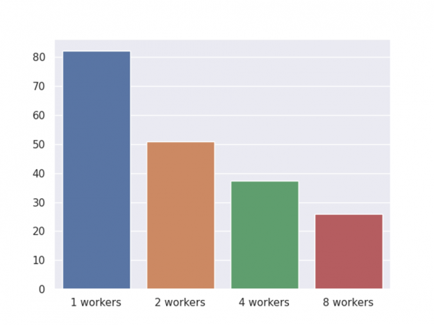
图 3 : GPU 集群端到端时间。
与之前一样,基准测试是在一台 NVIDIA DGX-1 服务器上执行的,该服务器有 8 个 V100 gpu 和两个 20 核的 Xeon E5 – 2698 v4 cpu ,并进行一轮训练、 shap 值计算和推理。此外,我们还共享了两种内存使用优化,图 4 描述了总体内存使用比较。
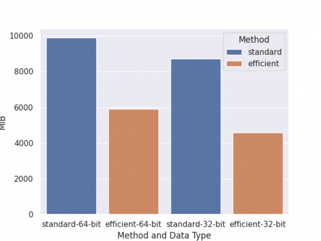
左两列是 64 位数据类型训练的内存使用情况,右两列是 32 位数据类型训练的内存使用情况。标准是指使用正常的数据矩阵和预测函数进行训练。有效的方法是使用 DaskDeviceQuantileDMatrix 和 inplace_predict.
Scikit 学习包装器
前面的章节考虑了“功能”接口的基本模型训练,但是,还有一个类似 scikit 学习估计器的接口。它更容易使用,但有更多的限制。在 XGBoost1 . 4 中,此接口与单节点实现具有相同的特性。用户可以选择不同的估计器,如 DaskXGBClassifier 用于分类,而 DaskXGBRanker 用于排名。查看参考资料以获得可用估算器的完整列表: https://xgboost.readthedocs.io/en/latest/python/python_api.html#module-xgboost.dask 。
概括
我们已经介绍了一个在 GPU 集群上使用 RAPIDS 库加速 XGBoost 的示例,它显示了使 XGBoost 代码现代化可以帮助最大限度地提高培训效率。通过 XGBoost Dask 接口和 RAPIDS ,用户可以通过一个易于使用的 API 实现显著的加速。尽管 XGBoost-Dask 接口已经达到了与单节点 API 的功能对等,但仍在继续开发,以便更好地与其他库集成,实现超参数调优等新功能。对于与 dask 接口相关的新功能请求,您可以在 XGBoost 的 GitHub 存储库 上打开一个问题。
要了解有关同时使用 Dask 和 RAPIDS 的更多信息,请查看 NVIDIA 2021 年达斯克分布式峰会上的演讲 。有关 RAPIDS 和 Dask 的概述,请收听 GPU 加速数据科学研讨会 。要深入了解基于代码的示例,请查看 辅导的 。