There’s an important technology that is commonly used in autonomous driving, medical imaging, and even Zoom virtual backgrounds: semantic segmentation. That’s the process of labelling pixels in an image as belonging to one of N classes (N being any number of classes), where the classes can be things like cars, roads, people, or trees. In the case of medical images, classes correspond to different organs or anatomical structures.
NVIDIA Research is working on semantic segmentation because it is a broadly applicable technology. We also believe that the techniques discovered to improve semantic segmentation may also help to improve many other dense prediction tasks, such as optical flow prediction (predicting the motion of objects), image super-resolution, and so on.
We have developed a new method for semantic segmentation that achieves record-setting state-of-the-art results in two common benchmarks: Cityscapes and Mapillary Vistas, as seen in the following tables. IOU is intersection over union, a metric that describes the accuracy of semantic prediction.
In Cityscapes, this method achieves 85.4 IOU on the test set, a sizable improvement over other entries, given how close each of those scores are to each other.
| Entry | IOU |
| Ours | 85.4 |
| Panoptic DeepLab | 85.2 |
| HRNet-OCR SegFix | 84.5 |
| iFlytek-CV | 84.4 |
| MoKu Lab | 84.3 |
With Mapillary, it achieves 61.1 IOU on the validation set with a single model, as compared to the next best result that used an ensemble to achieve 58.7.
| Entry | IOU |
| Ours | 61.1 |
| Panoptic Deeplab (ensemble) | 58.7 |
| DeepLabV3+ | 52.0 |
| Seamless | 50.4 |
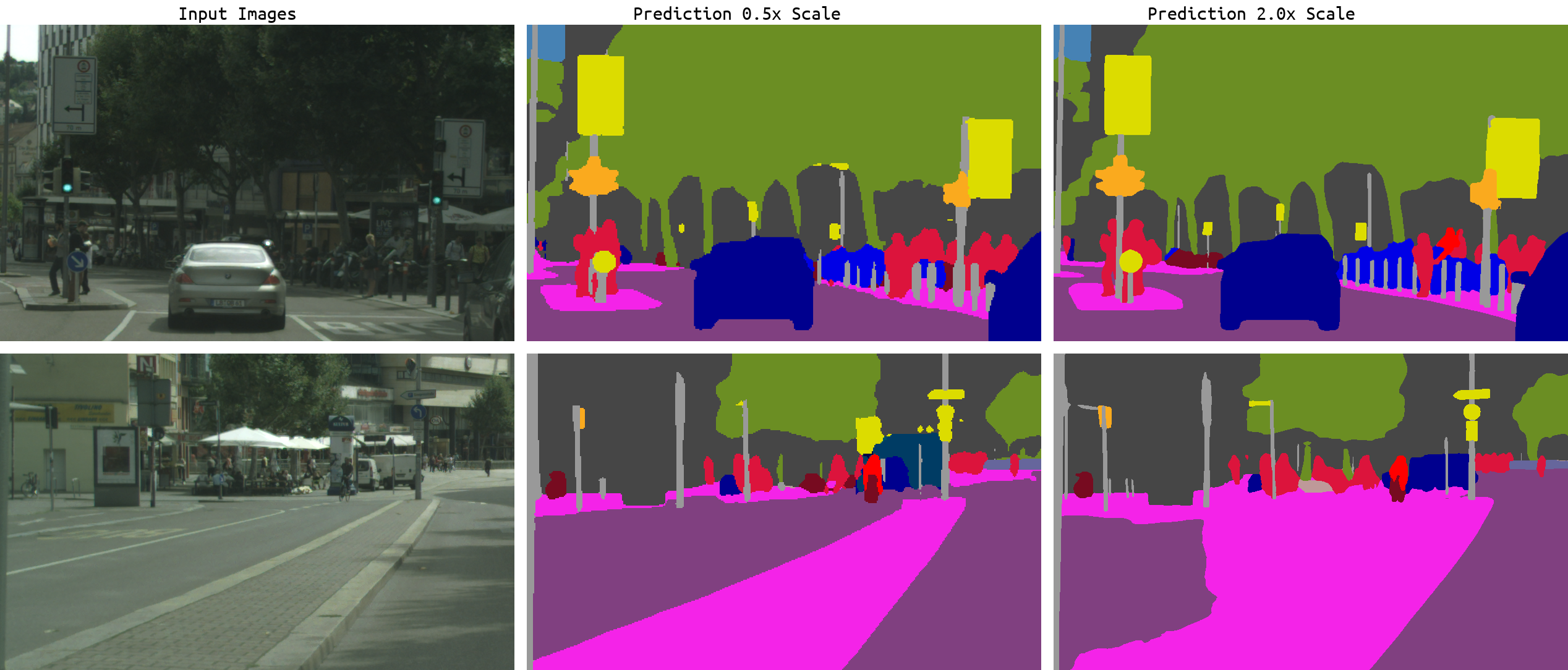
Prediction results
Research journey
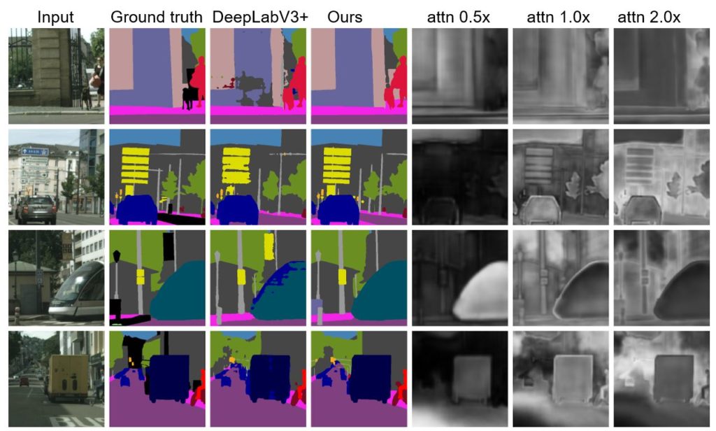
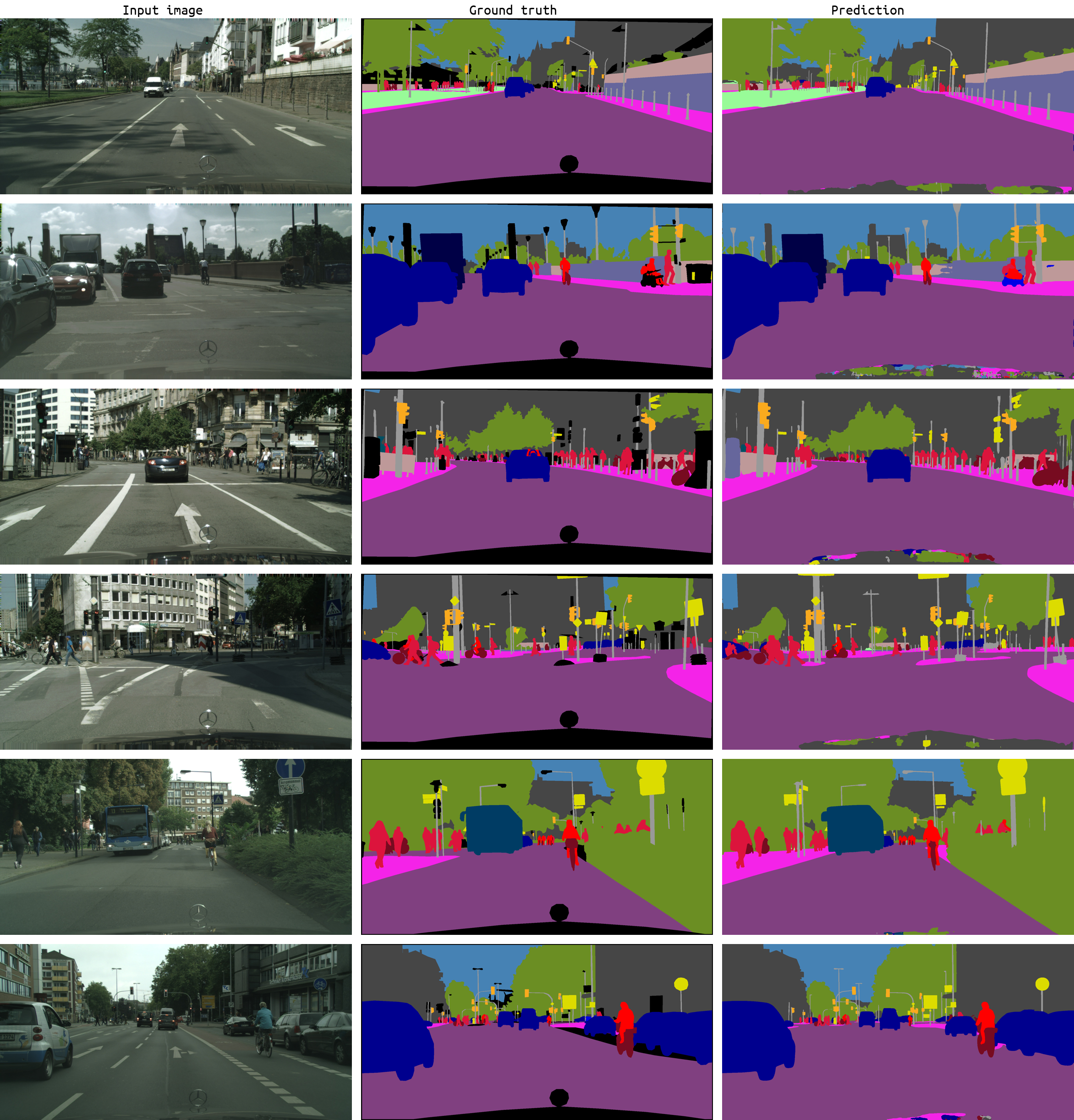
To develop this new method, we considered what specific areas of an image needed improvement. Figure 2 shows two of the biggest failure modes of current semantic segmentation models: errors with fine detail and class confusion.
In this example, two issues are present: fine detail and class confusion.
- The fine details of the posts in the first image are best resolved in the 2x scale prediction, but poorly resolved at 0.5x scale.
- The coarse prediction of the road compared to median segmentation is much better resolved at 0.5x scale than 2x scale, where there is class confusion.
Our solution performs much better on both issues, with the class confusion all but gone in the road and much smoother and consistent prediction of the fine detail.
After identifying these failure modes, the team experimented with many different strategies, including different network trunks (for example, WiderResnet-38, EfficientNet-B4, Xception-71), as well as different segmentation decoders (for example, DeeperLab). We decided to adopt HRNet as the network backbone and RMI as the primary loss function.
HRNet has been demonstrated to be well-suited to computer vision tasks as it maintains a 2x higher resolution representation than the previous network WiderResnet38. The RMI loss provides a way to have a structural loss without having to resort to something like a conditional random field. Both HRNet and RMI loss were helpful to address both fine detail and class confusion.
To further address the primary failure modes, we innovated on two approaches: multi-scale attention and auto-labelling.
Multi-scale attention
To achieve the best results, it is common practice in computer vision models to use multi-scale inference. Multiple image scales are run through the network and the results are combined with average pooling.
Using average pooling as a combination strategy treats all scales as equally important. However, fine detail is usually best predicted at higher scales and large objects are better predicted at lower scales, where the receptive field of the network is better able to understand the scene.
Learning how to combine multi-scale predictions at a pixel level can help to address this issue. There is prior work on this strategy, with Chen’s approach in Attention to Scale being the closest. In Chen’s method, attention is learned for all scales simultaneously. We refer to this as the explicit approach, shown in Figure 3.
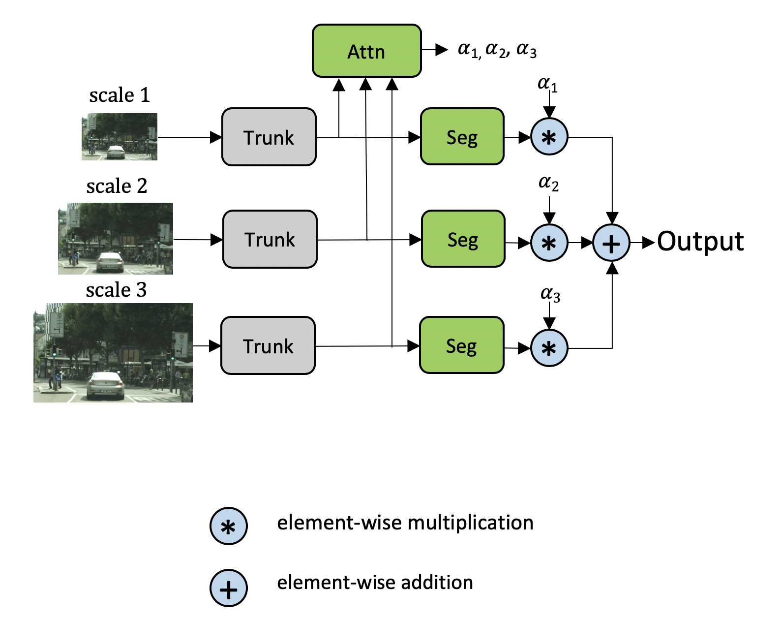
Motivated by Chen’s approach, we proposed a multi-scale attention model that also learns to predict a dense mask to combine multi-scale predictions together. However, in this method, we learn a relative attention mask to attend between one scale and the next higher scale, as shown in Figure 4. We refer to this as the hierarchical approach.

The primary benefits to this approach are as follows:
- The theoretical training cost is reduced over Chen’s method by ~4x.
- While training happens with only pairs of scales, inference is flexible and can be done with any number of scales.
| Train scales | Eval scales | Mapillary val IOU | Training Cost | Minibatch time (sec) | |
| Baseline single scale | 1.0 | 1.0 | 47.7 | 1.00x | 0.8 |
| Baseline avgpool | 1.0 | 0.5,1.0,2.0 | 49.4 | 1.00x | 0.8 |
| Explicit | 0.5,1.0,2.0 | 0.5,1.0,2.0 | 51.4 | 5.25x | 3.1 |
| Hierarchical (Ours) | 0.5,1.0 | 0.5,1.0,2.0 | 51.6 | 1.25x | 1.2 |
| Hierarchical (Ours) | 0.5,1.0 | 0.25,0.5,1.0,2.0 | 52.2 | 1.25x | 1.2 |
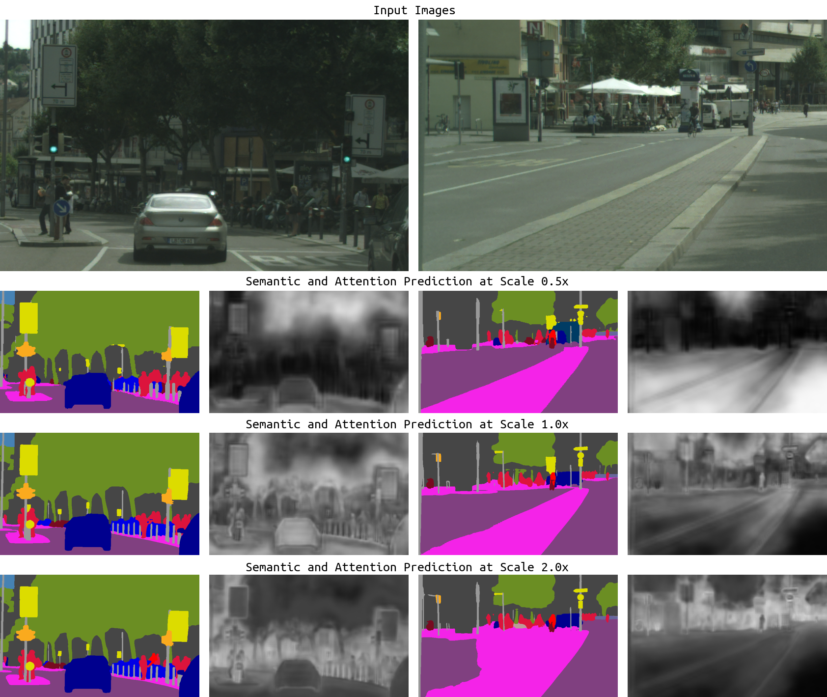
Some examples of our method, along with the learned attention mask, are shown in Figure 5. For the fine posts in the image on the left, there is little attention to the 0.5x prediction, but a very strong attention to the 2.0x scale prediction. Conversely, for the very large road/divider region in the image on the right, the attention mechanism learns to most leverage the lower scale (0.5x) and much less of the erroneous 2.0x prediction.
Auto-labelling
A common approach to improving semantic segmentation results with Cityscapes is to leverage the large set of coarse data. This data is roughly 7x as large as the baseline fine data. Previous SOTA approaches to Cityscapes used coarse labels as-is and either use the coarse data for pretraining the network or mix it in with the fine data.
However, the coarse labels present a challenge because they are noisy and imprecise. The ground truth coarse labels are shown in Figure 6 as ‘Original coarse label’.
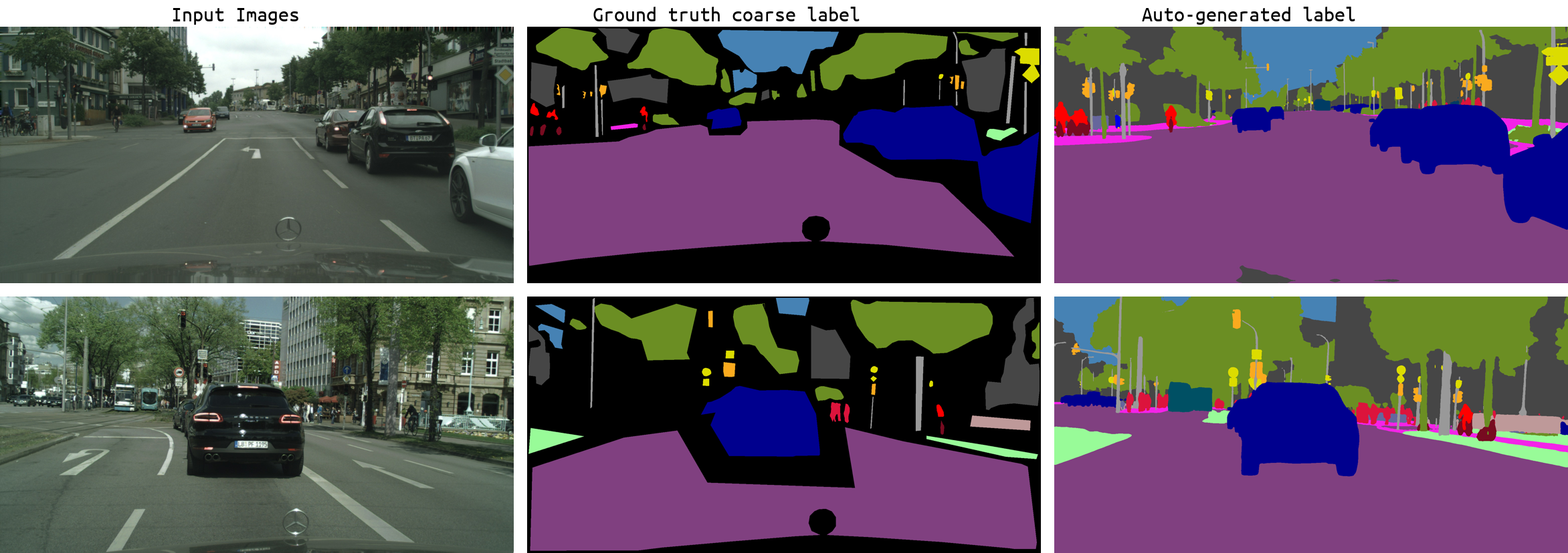
Inspired by recent work, we pursued auto-labelling as a means to generate much richer labels to fill in the labelling gaps in the ground truth coarse labels. Our generated auto-labels show much finer detail than the baseline coarse labels as seen in Figure 6. We believe that this helps generalization by filling in the gaps in the data distribution for long-tail classes.
A naive approach to using auto-labelling, such as using the multi-class probabilities from a teacher network to guide the student, would be very costly in disk space. Generating labels for the 20,000 coarse images, which are all 1920×1080 in resolution across 19 classes would cost roughly 2 TB of storage. The biggest impact of such a large footprint would be reduced training performance.
We used a hard thresholding approach instead of a soft one to vastly reduce the generated label footprint from 2 TB to 600 MB. In this approach, teacher predictions with probability > 0.5 are valid, and predictions with lower probability are treated as an ‘ignore’ class. Table 4 shows the benefit of adding the coarse data to the fine data and training a new student with the fused dataset.
| Dataset | Cityscales Val IOU | Benefit |
| Fine + ground truth coarse labels | 85.4 | – |
| Fine + auto-generated coarse labels | 86.3 | 0.9 |
Final details
This model was trained using the PyTorch framework with automated mixed precision training with fp16 Tensor Cores across four DGX nodes.
For more information, see the paper, Hierarchical Multi-Scale Attention for Semantic Segmentation, and the code in the NVIDIA/semantic-segmentation GitHub repo, where you can run pretrained models or train your own.
To learn more about projects like this, see Research at NVIDIA.
