
This post was originally published on the RAPIDS AI blog.
There is a wide range of graph applications and algorithms that I hope to discuss through this series of blog posts, all with a bias toward what is in RAPIDS cuGraph. I am assuming that the reader has a basic understanding of graph theory and graph analytics. If there is interest in a graph analytic primer, please leave me a comment below. It should also be noted that I approach graph analysis from a social network perspective and tend to use the social science theory and terms, but I have been trying to use ‘vertex’ rather than ‘node.’
Every RAPIDS cuGraph 0.7 release adds new features. Of interest to this discussion is the expansion of the Jaccard Similarity metric to allow for comparisons of any pair of vertices, and the addition of the Overlap Coefficient algorithm. Those two algorithms fall into the category of similarity metrics and lead to the topic of this blog, which is to discuss the difference between the two algorithms and why I think one is better than the other. Let’s start with a quick introduction to the similarity metrics (warning math ahead).
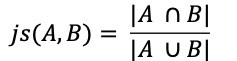
The Jaccard Similarity, also called the Jaccard Index or Jaccard Similarity Coefficient, is a classic measure of similarity between two sets that was introduced by Paul Jaccard in 1901. Given two sets, A and B, the Jaccard Similarity is defined as the size of the intersection of set A and set B (i.e. the number of common elements) over the size of the union of set A and set B (i.e. the number of unique elements).
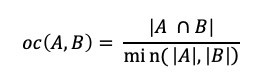
The Overlap Coefficient, also known as the Szymkiewicz–Simpson coefficient, is defined as the size of the union of set A and set B over the size of the smaller set between A and B.
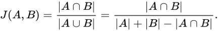
When applying either of the similarity metrics in a graph setting, the sets are typically comprised of the neighbors of the vertex pair being compared. The neighbors of a vertex v, in a graph (V,E) is defined as the set, U, of vertices connected by way of an edge to vertex v, or N(v) = {U} where v ∈V and ∀ u ∈ U ∃ edge(v,u) ∈ E. Computing the size of the union, | A U B |, can be computationally inexpensive since we only want the size and not the actual elements. The size of the union| A U B | can be computed with |A| + |B| — | A intersect B |.
There is a wide range of applications for similarity scoring and it is important to cover a few of them before getting into comparing the two algorithms. Let’s start with something that I’m sure a lot of the reader are familiar with, and that is recommending people to connect with on social media. What I am going to present is a very simplistic approach to the problem — most social networking sites use a much more advanced version that usually includes some type of community detection. But first, even more background …
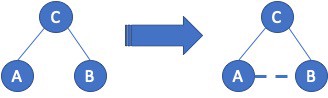
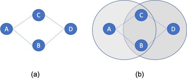
Within the field of social network analysis, there is the concept of Triadic Closure, which was first introduced by sociologists Georg Simmel in 1908. Given three people, A, B, and C, see Figure 1; if A and C are friends (connected), and B and C are friends, then there is a high probability that A and B will connect. That probability is so high that Granovetter, in his 1973 work on weak-ties, deemed the missing link as the “forbidden triad”, which meant that for Granovetter’s application that you could infer a connection between A and B. For our recommendation application, this means that we need to find those unconnected A — B pairs since there is a high change that those users will become friends — it is always good to recommend something that the user will accept.
Now back to the application: the basic process starts by first computing the similarity metric (Jaccard or Overlap Coefficient) for all vertex pairs connected by an edge. Then for a given vertex (example, vertex A) find their neighbors with the highest similar score and recommend neighbors of B that are missing from A. As mentioned, this is a very simple view since there is a range of options for applying additional weights, like only looking within community clusters, that could be added to better select recommendations that will be accepted. The application of triadic closure and similarity should be apparent to anyone that uses social media since those tools remind you constantly that you should connect to a friend of friends. Note that this approach does not work for vertices with a single connection, also called a satellite, since their similarity score will be zero. But for satellites it is easy to just recommend all connections from their sole neighbor.
The problem with the previous approach is that not all recommendations can come from solely looking at directly connected vertex pairs. Therefore, being able to compute similarity scores between any pair of vertices is important. This was a limitation of the initial cuGraph Jaccard implementation and what has been addressed in cuGraph release 0.7. Consider figure 2 below. Looking at the Jaccard similarity score between connected vertices A and B, the neighbors of A are {B, C}, and for B are {A, D}. Hence the Jaccard score is js(A, B) = 0 / 4 = 0.0. Even the Overlap Coefficient yields a similarity of zero since the size of the intersection is zero. Now looking at the similarity between A and D, where both share the exact same set of neighbors. The Jaccard Similarity between A and D is 2/2 or 1.0 (100%), likewise the Overlap Coefficient is 1.0 size in this case the union size is the same as the minimal set size.
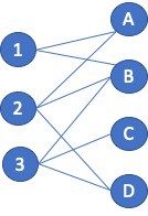
Continuing with the social network recommender example, the application should recommend that vertices A and D connect since they share the same set of neighbors. But non-connected vertex pair similarity is used in other applications as well. Consider a product recommendation system that is using a bipartite graph. One vertex type is Users and the other type is Product. The goal is to not find similarities between Users and Products as that is a different analytic but to find similarities between Users and other Users so that additional products can be recommended. The process is similar to that mentioned above; the vertices being compared are just not directly connected. Looking at the example figure (Figure 3) and focusing on User 1. User 1 neighbors are {A, B}, User 2 are {A, B, D} , and User 3 is {B. D}. The Jaccard Similarity in this case is 1-to-2 = 2 / 3 = 0.66, and between 1 and 3 = 1 / 3 = 0.33. Since User 1 and 2 both purchased products A and B, the application should recommend to User 1 that they also purchase product D.
Why I prefer the overlap coefficient
If the Jaccard similarity score is so useful, why introduce the Overlap Coefficient in cuGraph? Let’s look at the same example but using the Overlap Coefficient. Comparing User 1 to User 2 = 2 /2 = 1.0. And comparing User 1 to User 3 = 1 /2 = 0.5. The similarity between User 1 and User 2 is still the highest, but the fact the score is 1.0 indicated that the set of neighbors of User A is a complete subset of User 2. That type of insight is one of the benefits of the Overlap Coefficient.
In my opinion, the Jaccard Similarity is a very powerful analysis technique, but it has a major drawback when the two sets being compared have different sizes. Consider two sets, A and B, where both sets contain 100 elements. Now assume that 50 of those elements are common across the two sets. The Jaccard Similarity is js(A, B) = 50 / (100 + 100 – 50 ) = 0.33. Now if we increase set A by 10 elements and decrease set B by the same amount, all while maintaining 50 elements in common, the Jaccard Similarity remains the same. And there is where I think Jaccard fails: it has no sensitivity to the sizes of the sets. The following figure highlights how the Jaccard and Overlap Coefficient change as the set sizes are change but the intersection size remains that same.
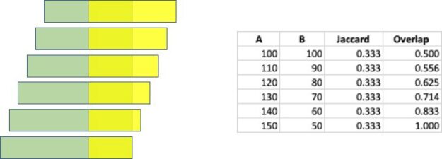
The use of the smaller set size as the denominator makes it so that the score provides an indication of how much of the smaller set is within the larger. That provides insight into whether one set is an exact subset of the larger set. Look back at the example described above, and illustrated above, using the Overlap Coefficient it is easy to see to what degree set B is contained within set A.
Conclusion
<warning, the following is just my opinion>
Jaccard might be better known than the Overlap Coefficient and that might play into why Jaccard is more widely used. The unfamiliarity with Overlap Coefficient might explain why it is not in the NetworkX package. Nevertheless, in my opinion, the Overlap Coefficient can provide better insight into how similar two vertices are — really, how similar the set of neighbors are. By knowing the sizes of each set, an analyst can easily know if one set is a proper subset (full contained) in the other set, which is something that is not apparent using Jaccard.
I also think there is a fundamental flaw in how we derive the set for similarity computation when the vertex pairs are connected by an edge. Consider the 5-clique shown below, figure 5. Since every vertex is connected to every other vertex, I (you) would assume that the similarity scores would be 1.0, exact similarity. However, because of the way the sets are created, for both Jaccard and the Overlap Coefficient, the score for vertex pairs connected by an edge can never be equal to 1.0.
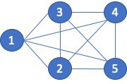
Let’s compare vertex 1 to vertex 2. The neighbors of 1 are {2, 3, 4, 5} and the neighbors of 2 are {1, 3, 4, 5}. The Jaccard score is then: 3 / 5 or 0.6. The Overlap Coefficient is 3 /4 or 0.75.
While those similarity scores are mathematically correct according to the algorithm, the resulting similarity score do not match what I would except for a clique. The issue is that the vertex pairs being compared are reflected in the neighborhood sets. Rephrasing that statement, vertex 1 appears in vertex 2’s neighbor set. Likewise, vertex 2 appears in vertex 1’s neighbor. The fact that the vertices being compared appear in the associative set prevents the sets from ever matching. In my opinion, the vertices being compared should not be part of the sets being evaluated.
A solution to this problem would be to build the sets differently or modify the similarity algorithm. The algorithm modification might be computationally easier. The change would be to subtract 1 from the size of each set on the union, not the intersection.
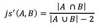
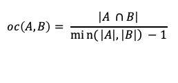
For the clique example, the similarity scores would then be:
js(1, 2) = 3 / (5–2) = 3/3 = 1.0. and
oc(1, 2) = 3 / (4–1) — 3/3 = 1.0.
Now, it could be that the results are correct and that my expectation are wrong. But this is just my opinion 🙂
About me
Brad Rees leads the RAPIDS cuGraph team at NVIDIA where he directs and develops graph analytic solutions. He has been designing, implementing, and supporting a variety of advanced software and hardware systems for over 30 years. Brad specializes in complex analytic systems, primarily using graph analytic techniques for social and cyber network analysis, and has been working on variety of advanced software and hardware systems for over 30 years. His technical interests are in HPC, machine learning, deep learning, and graph. Brad has a Ph.D. in Computer Science from the Florida Institute of Technology.
Some references
M. S. Granovetter, “The strength of weak ties,” The American Journal of Sociology, vol. 78, no. 6, pp. 1360–1380, 1973.
Thanks to Corey Nolet.
