
The 25.08 release of RAPIDS continues to push the boundaries toward making accelerated data science more accessible and scalable with the addition of several new features, including:
- Two new profiling tools for troubleshooting cuml.accel code
- Support for larger, more complex data in the Polars GPU engine
- New algorithm support in cuML and cuml.accel
- An update on CUDA version support
Learn more about the new features below.
New profiling tools for cuML’s zero code change accelerator
The 25.08 release brings the addition of two new profiling options to cuml.accel. Similar to the profiler that was previously released for cudf.pandas, these new profiling features help users understand which operations are accelerated by cuML on the GPU, which fall back to running on the CPU, and how long these operations take. This can be useful for users trying to understand current performance bottlenecks in their machine learning workflows.
First, we introduced a function-level profiler. This profiler shows users all of the operations in a given script or cell that were run on the GPU vs. CPU. It also shows the amount of time each function took on each.
There are two ways to use the function-level profiler. If running a Jupyter or IPython notebook, users can call %%cuml.accel.profile after cuml.accel has already been loaded and profile an entire cell:
%%cuml.accel.profile


from sklearn.linear_model import Ridge
from sklearn.datasets import make_regression


X, y = make_regression(n_samples=100)


# Fit and predict on GPU
ridge = Ridge(alpha=1.0)
ridge.fit(X, y)
ridge.predict(X)


# Retry, using an unsupported hyperparameter
ridge = Ridge(positive=True)
ridge.fit(X, y)
ridge.predict(X)
The output of this cell contains the profile result:
cuml.accel profile
┏━━━━━━━━━━━━━━━┳━━━━━━━━━━━┳━━━━━━━━━━┳━━━━━━━━━━━┳━━━━━━━━━━┓
┃ Function      ┃ GPU calls ┃ GPU time ┃ CPU calls ┃ CPU time ┃
┡━━━━━━━━━━━━━━━╇━━━━━━━━━━━╇━━━━━━━━━━╇━━━━━━━━━━━╇━━━━━━━━━━┩
│ Ridge.fit     │         1 │  141.2ms │         1 │      3ms │
│ Ridge.predict │         1 │   31.5ms │         1 │   97.3µs │
├───────────────┼───────────┼──────────┼───────────┼──────────┤
│ Total         │         2 │  172.7ms │         2 │    3.1ms │
└───────────────┴───────────┴──────────┴───────────┴──────────┘
Not all operations ran on the GPU. The following functions required CPU fallback for the following reasons:
* Ridge.fit
  - `positive=True` is not supported
* Ridge.predict
  - Estimator not fit on GPU
The function-level profiler can also be called on a Python script using the --profile flag from the CLI:
python -m cuml.accel --profile script.py
The second profiler is a line-level profiler, showing users where each piece of code is executed line-by-line. Like the function-level profiler, the line-level profiler can be called within a notebook with %%cuml.accel.line_profile.
%%cuml.accel.line_profile


from sklearn.linear_model import Ridge
from sklearn.datasets import make_regression


X, y = make_regression(n_samples=100)


# Fit and predict on GPU
ridge = Ridge(alpha=1.0)
ridge.fit(X, y)
ridge.predict(X)


# Retry, using an unsupported hyperparameter
ridge = Ridge(positive=True)
ridge.fit(X, y)
ridge.predict(X)
cuml.accel line profile
┏━━━━┳━━━┳━━━━━━━━━┳━━━━━━━┳━━━━━━━━━━━━━━━━━━━━━━━━━━━━━━━━━━━━━━━━━━━━━━┓
┃  # ┃ N ┃    Time ┃ GPU % ┃ Source                                       ┃
┡━━━━╇━━━╇━━━━━━━━━╇━━━━━━━╇━━━━━━━━━━━━━━━━━━━━━━━━━━━━━━━━━━━━━━━━━━━━━━┩
│  1 │ 1 │       - │     - │ from sklearn.linear_model import Ridge       │
│  2 │ 1 │       - │     - │ from sklearn.datasets import make_regression │
│  3 │   │         │       │                                              │
│  4 │   │         │       │                                              │
│  5 │ 1 │   1.1ms │     - │ X, y = make_regression(n_samples=100)        │
│  6 │   │         │       │                                              │
│  7 │   │         │       │                                              │
│  8 │   │         │       │ # Fit and predict on GPU                     │
│  9 │ 1 │       - │     - │ ridge = Ridge(alpha=1.0)                     │
│ 10 │ 1 │ 174.2ms │  99.0 │ ridge.fit(X, y)                              │
│ 11 │ 1 │   5.2ms │  99.0 │ ridge.predict(X)                             │
│ 12 │   │         │       │                                              │
│ 13 │   │         │       │                                              │
│ 14 │   │         │       │ # Retry, using an unsupported hyperparameter │
│ 15 │ 1 │       - │     - │ ridge = Ridge(positive=True)                 │
│ 16 │ 1 │   4.5ms │   0.0 │ ridge.fit(X, y)                              │
│ 17 │ 1 │ 172.7µs │   0.0 │ ridge.predict(X)                             │
│ 18 │   │         │       │                                              │
└────┴───┴─────────┴───────┴──────────────────────────────────────────────┘
Ran in 185.6ms, 96.4% on GPU
The line profiler can also be called via the --line-profile flag from the command line:
python -m cuml.accel --line-profile script.py
With these new profiling capabilities, cuml.accel provides users with more tools to make accelerating and debugging machine learning code even easier.
Process larger, more complex data with the Polars GPU engine powered by NVIDIA cuDF
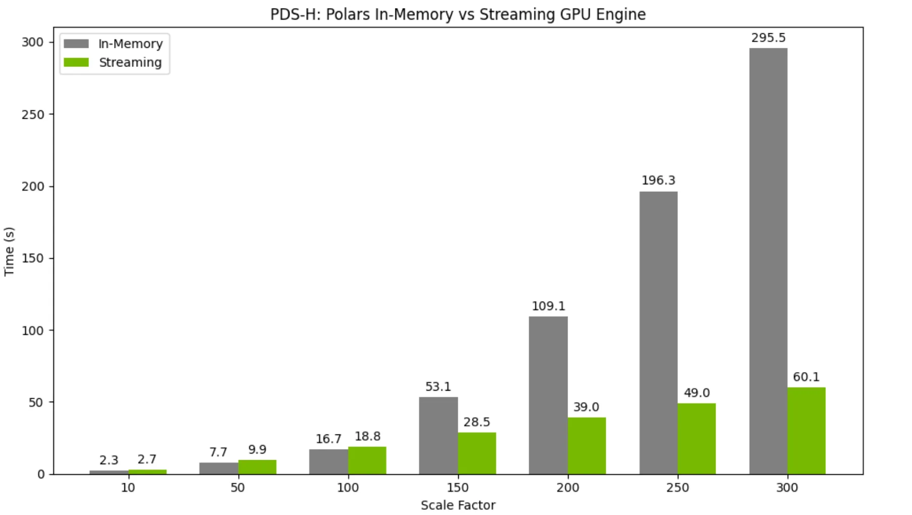
Work with datasets larger than GPU memory with the new default streaming executor
The streaming execution mode that was introduced as an experimental feature in 25.06 is now the default in the Polars GPU engine. This new executor takes advantage of data partitioning to allow datasets much larger than VRAM (GPU memory) to be processed efficiently. The streaming executor can still fall back to in-memory execution for any unsupported operations, but as of the 25.08 release, streaming execution supports almost all of the operators that are supported for in-memory GPU execution. This unlocks substantial performance and scalability improvements.
For smaller datasets, using the streaming execution mode on a single GPU incurs a very minor performance overhead when compared to using the in-memory engine. However, as dataset size grows and begins to exceed GPU memory, the streaming executor provides massive speedups compared to the in-memory engine.
For more information on the Polars GPU streaming executor, visit our documentation.
Keep complex data like structs and string operations on the GPU
The Polars GPU engine now supports struct data in columns. Previously, any operations involving structs would fall back to CPU execution, but with the latest release all of these operations are now GPU-accelerated for improved performance:
>>> import polars as pl
... ratings = pl.LazyFrame(
...     {
...         "Movie": ["Cars", "IT", "ET", "Cars", "Up", "IT", "Cars", "ET", "Up", "ET"],
...         "Theatre": ["NE", "ME", "IL", "ND", "NE", "SD", "NE", "IL", "IL", "SD"],
...         "Avg_Rating": [4.5, 4.4, 4.6, 4.3, 4.8, 4.7, 4.7, 4.9, 4.7, 4.6],
...         "Count": [30, 27, 26, 29, 31, 28, 28, 26, 33, 26],
...     }
... )
... ratings.select(pl.col("Theatre").value_counts()).collect(engine=pl.GPUEngine(raise_on_fail=True))
...
shape: (5, 1)
┌───────────┐
│ Theatre     │
│ ---         │
│ struct[2]   │
╞═════════==╡
│ {"NE",3}    │
│ {"ND",1}    │
│ {"ME",1}    │
│ {"SD",2}    │
│ {"IL",3}    │
└───────────┘
Additionally, the Polars GPU engine now supports a substantially expanded set of string operators, for example:
>>> ldf = pl.LazyFrame({"foo": [1, None, 2]})
>>> ldf.select(pl.col("foo").str.join("-")).collect(engine=gpu_engine)
shape: (1, 1)
┌─────┐
│ foo  │
│ ---  │
│ str  │
╞═════╡
│ 1-2  │
└─────┘
>>> ldf = pl.LazyFrame({
...     "lines": [
...         "I Like\nThose\nOdds",
...         "This is\nThe Way",
...     ]
... })
... ldf.with_columns(
...     pl.col("lines").str.extract(r"(T\w+)", 1).alias("matches"),
... ).collect(engine=pl.GPUEngine(raise_on_fail=True))
...
shape: (2, 2)
┌─────────┬──────┐
│ lines   ┆ matches │
│ ---     ┆ ---     │
│ str     ┆ str     │
╞═════════╪══════╡
│ I Like  ┆ Those   │
│ Those   ┆         │
│ Odds    ┆         │
│ This is ┆ This    │
│ The Way ┆         │
└─────────┴──────┘
The expansion of datatype support further strengthens the capabilities of the Polars GPU engine, accelerating the delivery of the most common end user functionality.
New algorithms supported in cuML: Spectral Embedding, LinearSVC, LinearSVR, and KernelRidge
With the 25.08 release, cuML has added a Spectral Embedding algorithm for dimensionality reduction and manifold learning. Spectral Embedding is an approach which uses the eigenvalues and eigenvectors of a similarity graph to embed high-dimensional data into a lower-dimensional space.
The API for the new Spectral Embedding algorithm in cuML matches that of the Spectral Embedding implementation in scikit-learn:
from cuml.manifold import SpectralEmbedding
import cupy as cp
from sklearn.datasets import fetch_openml


# (70000, 784) -> (70000, 2)
mnist = fetch_openml('mnist_784', version=1)
X, y = mnist.data, mnist.target.astype(int)


spectral = SpectralEmbedding(n_components=2, n_neighbors=None, random_state=42)
embedding = spectral.fit_transform(cp.asarray(X, order='C', dtype=cp.float32))
Additionally, cuml.accel now accelerates several new algorithms with zero code changes. LinearSVC and LinearSVR estimators were added in the 25.08 release, which means that all estimators within the support vector machine family are now a part of cuml.accel.
KernelRidge was also added to cuml.accel, bringing another popular regression algorithm under the zero code change umbrella.
For more information on the algorithms that are supported today, check out our full documentation.
Deprecation of CUDA 11 support
Beginning with the 25.08 release, we dropped support for CUDA 11, which includes all containers, published packages, and the ability to build from source. Users who want to continue running CUDA 11 may pin to RAPIDS version 25.06.
Visit the RAPIDS documentation to learn more.
Conclusion
The NVIDIA RAPIDS 25.08 release offers a substantial leap forward in accelerating and optimizing data science workflows. With the introduction of the cuml.accel profiler, developers now have powerful tools to diagnose and improve the performance of their machine learning code. Updates to the Polars GPU engine like the streaming executor and expanded data type support enable efficient processing of large datasets, enhancing scalability and performance. Additionally, the inclusion of new algorithms in cuML further streamlines the machine learning ecosystem. These developments collectively contribute to making accelerated data science more accessible and efficient for users. For a deeper dive into all the new features and improvements, be sure to visit the RAPIDS documentation.
We welcome your feedback on GitHub. You can also join the 3,500+ members of the RAPIDS Slack community to talk GPU-accelerated data processing.
If you’re new to RAPIDS, check out these resources to get started and take our Accelerate Data Science Workflows with Zero Code Changes course for free. To learn more about accelerated data science, explore our DLI Learning Path and enroll in a hands-on course, such as Best Practices in Feature Engineering for Tabular Data With GPU Acceleration.