By Yi Dong, Alex Volkov, Miguel Martinez, Christian Hundt, Alex Qi, and Patrick Hogan – Solution Architects at NVIDIA.
Quantitative finance is commonly defined as the use of mathematical models and large datasets to analyze financial markets and securities. This field requires massive computational effort to extract knowledge from raw data.
Many scientific toolkits are available for processing data. The data is ingested as scalar values or in array form organized in data frames. This approach allows for convenient high-level manipulation of information and significantly improves productivity of quantitative finance scientists and developers.
The ever-increasing amount of collected data, however, imposes novel challenges not being addressed by established scientific libraries. Historically, those libraries were optimized for single-threaded execution on traditional CPUs. There exist multiple barriers to widespread GPU adoption in financial services.
- Efficient and easy to use GPU implementations for common algorithms in quantitative finance are lacking. Massively parallel accelerators have been widely adopted for number crunching due to their vast compute capability, highly competitive compute-to-energy ratio, and unprecedented memory bandwidth.This potential has not been leveraged by mainstream applications for quantitative analysis.
- Development cycles of financial applications are delayed by the time-consuming processing of compute-bound tasks. This includes model selection or parameter tuning on huge datasets. The highly regular structure of linear algebra primitives frequently used in statistical models allows for an enormous reduction of execution time when using GPUs. Rapid execution and frequent alteration is crucial for sufficient exploration of the model space, and performance is key for successful and fast algorithmic development.
- Distributed and asynchronous processing of interdependent tasks across multiple compute units (CPUs, GPUs, or even compute nodes) is challenging. It involves complex communication among tasks and non-trivial synchronization patterns. The manual design of aforementioned dependencies is time-consuming and error-prone. Ideally, this layer of complexity should be hidden from the developer.
Banks, hedge funds, and other financial services industry firms are notoriously secretive when it comes to algorithms and technology that might give them an edge in the markets. Growing adoption of GPU accelerated computing is unfortunately kept as a secret.
Our work with clients and experiences in the industry identified a need for concise and comprehensible examples of simple Python programs embedded in interactive notebooks. High performance implementations of well-known, established algorithms such as technical indicators can be used by data scientists or quants as templates for ongoing innovation and improvement of their own processing pipeline.
Under the gQuant umbrella, we have gathered a variety of open-source GPU accelerated examples for quantitative analyst tasks. It provides a coherent set of examples for researchers and data scientists to accelerate their workflows using GPUs.
More advanced examples include demonstrations of how to compose dataframe-flow driven graphs to accelerate entire workflows. These workflows can be organized at a high level and enable code portability across different hardware configurations. It has never been this easy to write and share simple yet efficient code in the FSI domain.
The dynamic distribution of asynchronous and overlapping tasks across multiple GPUs spanning several nodes is seamlessly facilitated by Dask-cuDF — a GPU-aware Dask extension for RAPIDS. Dask-cuDF organizes and simplifies data transfers of cuDF data frames and the lazy execution of tasks being encoded in an underlying dependency graph. This includes the pruning of redundant computations and the elision of unused intermediate results.
The gQuant repository contains a variety of detailed code samples that demonstrate the value of GPU-accelerated data science and empowers developers to contribute ground-breaking applications in the financial domain. For example, see Figure 1, which implements the relative strength index function. The gQuant examples are implemented on top of RAPIDS — a well established open-source library for CUDA-accelerated data science. The majority of functionality leverages highly optimized cuDF primitives while, for some functions, we implemented task specific GPU acceleration using Numba. The initial release demonstrates acceleration of 36 technical indicator computations frequently being used in financial quantitative analysis.

We also built examples that show how easy it is to build a full end-to-end workflow using a dataframe-flow that organizes a quant’s workflow as an acyclic directed graph (Figure 2). Each work unit becomes a node that receives dataframes as inputs from the parent nodes, validates the dataframes, computes the output dataframe(s), and passes its output(s) to the child nodes. The edges connecting the nodes show the direction of flow of the dataframe. Several of the examples are essentially a bundle of dataframe processing nodes that applies to the quants’ workflow. The initial set of examples includes “data loader”, “transformation”, “strategy”, “backtest”, and “analysis” node categories. The functionality of the nodes have an interface API, thus the nodes are decoupled from each other, making it easy for a data scientist to extend functionality with their own implementations.

Inside each node, the expected input dataframe entries (e.g., column names and types) are defined, and nodes output dataframe entries after the computation. Before the computation happens, validation is performed by traversing the graph to check the static types of inputs and outputs. Based on the node’s column name/type computation results, the set of compatible nodes can be determined. This reduces the complexity of wiring the graph.
Organizing the computation as a graph has a few other benefits. The graph structure is fully described and serialized to a yaml file that can be shared among team members. Each node can be serialized into a cache file on the file system or in a variable, and a sub-graph can be computed by loading those cached node states. This helps to remove the computation redundancy if multiple iterations of a sub-graph computation are required in the workflow. Other graph optimization techniques can be used naturally to optimize the performance.
The examples in gQuant will work with either cuDF dataframes or Dask-cuDF dataframes without changing the rest of the code. Distributed computation is enabled automatically by leveraging the Dask-cuDF and Dask distributed libraries.