How to Get Started with Neural Shading for Your Game or Application

For the past 25 years, real-time rendering has been driven by continuous hardware improvements. The goal has always been to create the highest fidelity image possible within 16 milliseconds. This has fueled significant innovation in graphics hardware, pipelines, and renderers.

But the slowing pace of Moore’s Law mandates the invention of new computational architectures to keep pace with the growing demand of real-time applications. Similarly, as traditional graphics methods approach their limits, new novel techniques are required to achieve further improvements in visual fidelity and performance. This creates a fundamental challenge: How do we continue improving real-time rendering without relying solely on traditional hardware advancements?

Neural shading represents an exciting new approach—integrating trainable models directly into the graphics pipeline to achieve unprecedented quality and performance. This new technique leverages dedicated AI hardware, such as NVIDIA’s Tensor Cores, to run these neural networks efficiently in real-time. 

In this blog, we’ll help you understand the fundamentals and get started with this transformative technology.

What is neural shading?

At its core, neural shading simply means making part of the graphics pipeline trainable. This could operate on anything with parameters that you can train using machine-learning techniques, but most promising are small neural networks that are executed inline in shaders and work in tandem with the rest of the renderer.

These small networks can be executed extremely efficiently in real-time, especially with hardware acceleration available through technologies like cooperative vectors. On one hand, this squeezes more efficiency out of existing hardware and gets more complexity on screen without relying on transistors getting smaller. On the other hand, making shaders trainable is extremely useful in its own right—neural shaders can tackle problems that are quite challenging to solve with traditional workflows. This adds a practical new tool to your graphics toolbox that works today.

How does this change the approach?

Traditional engineering involves understanding, solving, coding, and executing problems. However, some problems lack solutions, or the solutions are too costly for real-time computation, especially in neural shading. This is where optimization helps. Instead of direct problem-solving, we use known inputs and outputs to train a tunable mathematical model, iteratively adjusting parameters until an approximate, practically useful solution is achieved.

Modern neural shading can leverage powerful tools like Slang, a shading language emerging as a key technology in game development. Hosted by Khronos, the standards body that develops and maintains APIs like OpenGL and Vulkan, Slang offers broad platform compatibility, targeting HLSL, SPIR-V, Metal, and more. It incorporates modern language constructs like generics and, crucially for neural shading, supports automatic differentiation (autodiff), which automates complex calculus.

SlangPy is a Python interface to Slang. It provides a comprehensive, moderately low-level graphics API, offering access to core graphics constructs like compute buffers and textures. Highly cross-platform (targeting D3D 12, Vulkan, CUDA, and Metal), SlangPy also features a functional API that enables direct calls to Slang shader functions from Python.

For hands-on learning, check out the Slang introduction lab from SIGGRAPH and downloadable lab materials. You can also watch the Slang Birds of a Feather session for community discussions and insights.

Where to start?: A simple mipmap example

Let’s start with a concrete example to illustrate the concepts: the problem of mipmap generation. Traditional mipmaps work well for color textures like albedo maps, which downsample nicely even with simple box filters. However, maps that represent geometry or topology typically downsample very poorly because you can’t apply the same simple filter to geometry—you can’t say that a peak next to a trough becomes a flat surface.

The naive approach causes artifacts with noisy specular highlights, inventing nonexistent surfaces. This long-studied problem has analytical solutions, such as Toksvig’s method, which filters normal maps by adjusting roughness based on normal variance in mipmap levels, accounting for geometric complexity at different scales.

While these analytical approaches work well for specific cases, they often require domain-specific knowledge and careful parameter tuning. Neural optimization offers a more general solution—we can generate mipmaps that minimize the difference between the downsampled rendering and a reference “ideal” mipmap, learning optimal representations without requiring explicit analytical derivations.

How the optimization works

The optimization process involves two phases:

1. Forward phase: Render the ideal output using traditional methods, generate an output, and then measure the difference between the ideal and generated outputs.

2. Backward phase: Calculate how to adjust the inputs to make the error smaller using automatic differentiation.

The key insight is that we can use Slang’s autodiff capabilities to automatically generate the backward derivatives of our entire rendering procedure at compile time. This is much faster and more convenient than manual differentiation, and it always keeps the backward derivative in sync when we change the forward code.

Here’s a simple example of how a developer might approach this in Slang. Note that this is an illustrative example, and it would need to be adapted to a specific use case before running, by providing the input texture data, and an implementation of the BRDF function.

// Define our trainable mipmap parameters
struct MaterialParameters
{
    GradOutTensor<float3, 2> albedo;
    GradOutTensor<float3, 2> normal;

};

// Our differentiable render function
[Differentiable]
float3 render(int2 pixel, MaterialParameters material, no_diff float3 light_dir, no_diff float3 view_dir)
{
    // Bright white light
    float light_intensity = 5.0;

    // Sample very shiny BRDF (it rained today!)
    float3 brdf_sample = sample_brdf( // assume we've implemented our BRDF elsewhere
               material.get_albedo(pixel),  // albedo color
               normalize(light_dir),        // light direction
               normalize(view_dir),         // view direction
               material.get_normal(pixel),  // normal map sample
               0.05,                        // roughness
               0.0,                         // metallic (no metal)
               1.0                          // specular
               );

    // Combine light with BRDF sample to get pixel colour
    return brdf_sample * light_intensity;
}

// Simple box filter downsampling function
float3 downsample(
int2 pixel, 
Tensor<float3, 2> source)
{
    float3 res = 0;
    res += source.getv(pixel * 2 + int2(0, 0));
    res += source.getv(pixel * 2 + int2(1, 0));
    res += source.getv(pixel * 2 + int2(0, 1));
    res += source.getv(pixel * 2 + int2(1, 1));
    return res * 0.25;
}

// Loss function comparing our mipmap to reference
[Differentiable]
float3 loss(
no_diff int2 pixel, 
no_diff float3 reference, 
MaterialParameters material, 
no_diff float3 light_dir, 
no_diff float3 view_dir)
{
    float3 color = render(pixel, material,
                          light_dir, view_dir);
    float3 error = color - reference;
    return error * error; // Squared error
}

And here’s how to call this code with Python/SlangPy:

import slangpy as spy
import pathlib

# Create a device and load the Slang module
device = spy.create_device(
    include_paths=[
        pathlib.Path(__file__).parent.absolute(),
    ]
)
module = spy.Module.load_from_file(device, "example.slang")

# Load some materials.
albedo_map = spy.Tensor.load_from_image(device, "PavingStones070_2K.diffuse.jpg", linearize=True)
normal_map = spy.Tensor.load_from_image(device, "PavingStones070_2K.normal.jpg", scale=2, offset=-1)
def downsample(source: spy.Tensor, steps: int) -> spy.Tensor:
    for i in range(steps):
        dest = spy.Tensor.empty(
            device=device, 
            shape=(source.shape[0] // 2, source.shape[1] // 2),
            dtype=source.dtype)
        module.downsample(spy.call_id(), source, _result=dest)
        source = dest
    return source

# Allocate a tensor for output + call the render function 
output = spy.Tensor.empty_like(albedo_map)
module.render(pixel = spy.call_id(),
              material = {
                    "albedo": albedo_map,
                    "normal": normal_map,
              },
              light_dir = spy.math.normalize(spy.float3(0.2, 0.2, 1.0)),
              view_dir = spy.float3(0, 0, 1),
              _result = output)

# Downsample the output tensor.
output = downsample(output, 2)

# Save it to a file
output_filename = "render_output.png"
output.save_to_image(output_filename)

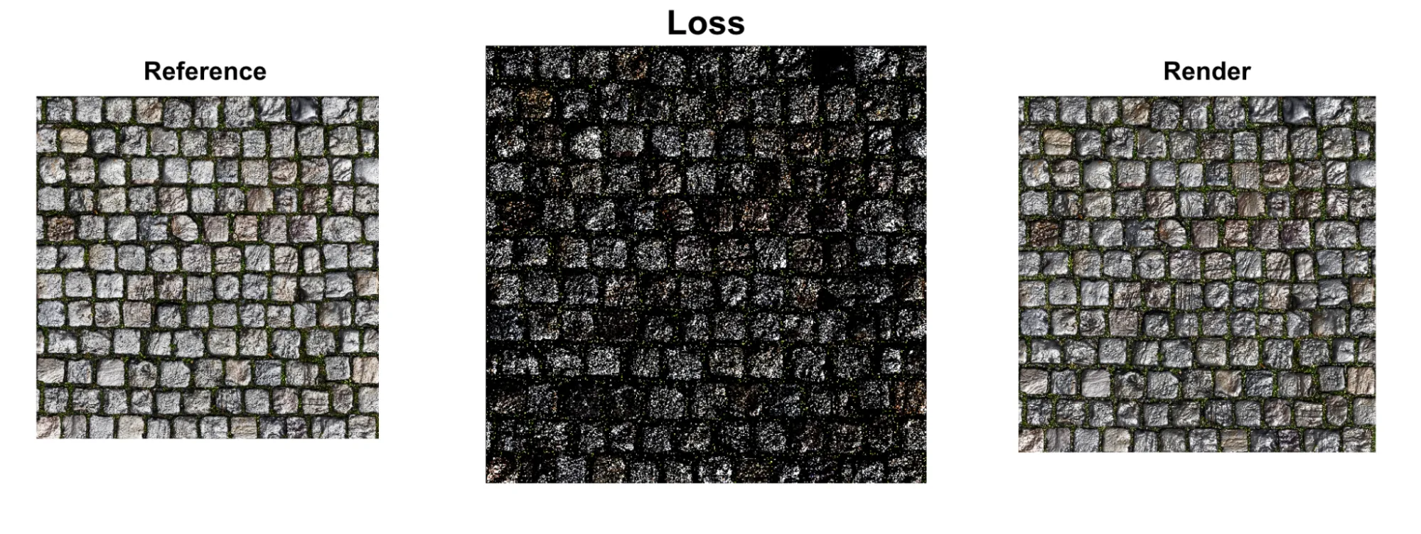
What we’ve done so far is take our original input texture, downsample it, and save it to a texture. We then need to calculate a result from some trainable parameters, and determine the difference between that result and our original. We’d like to train smaller input textures to achieve the same result as our full-resolution reference, so we’ll start by calculating the loss from those:

# Loss between downsampled full res output (the reference), 
# and result from quarter res inputs.
loss_output = spy.Tensor.empty_like(output)
module.loss(pixel = spy.call_id(),
         material = {
     	      "albedo": downsample(albedo_map, 2),
            "normal": downsample(normal_map, 2),
         },
         reference = output,
         light_dir = spy.math.normalize(spy.float3(0.2, 0.2, 1.0)),
         view_dir = spy.float3(0, 0, 1),
         _result = loss_output)

This code tells us how different our result is from what we want, but we don’t know how to adjust the parameters to reduce that loss. For that, we need to calculate the gradients, and this is where Slang’s autodiff will help us. Let’s add a function to the Slang code to do this:

void calculate_grads(
int2 pixel, 
MaterialParameters material, 
MaterialParameters ref_material) 
{ 
    float3 light_dir = random_direction(); // Assume we've implemented
    float3 view_dir = random_direction();  // a properly random direction
   // generator

    // Render the high-quality reference using our standard render function 
    float3 reference = render(pixel, ref_material, light_dir, view_dir); 

    // Backpropagate 
    bwd_diff(loss)(pixel, reference, material, light_dir, view_dir, 1.0); 

}

This new function uses the loss function that we defined to calculate gradients for each pixel in our material textures, by taking the derivative of that loss function with respect to each of those pixel inputs. Those gradients tell us how we need to update our input textures to reduce the loss.

The last step in the process is to update the input textures using those gradients, and then repeat, iteratively getting closer to our ideal. To do this, we’ll need one more Slang function to perform the update. For this example, we can use an extremely simple one, but real-world examples typically use more sophisticated optimizers like the Adam optimizer.

void optimizer_step(inout float3 parameter, float3 derivative, float learning_rate)
{ 
    parameter -= learning_rate * derivative; 
}

We can now repeat these two steps, calculating gradients and then using them to update our texture parameters, until we have trained a new, efficient mipmap. We do so with a simple Python loop:

for iteration in range(num_iterations):
    # Step 1: Calculate gradients via automatic differentiation
    module.calculate_grads(
        pixel=spy.call_id(),
        material=trainable_material,
        ref_material=reference_material
    )
    
    # Step 2: Update parameters using the optimizer
    module.optimizer_step(
        pixel=spy.call_id(),
        trainable_material["albedo"],
        learning_rate=learning_rate
    )
    # Repeat for normal map...

Note that the same rendering code that we use to calculate the color of our pixels is also used to train the mipmap parameters. The compiler automatically generates the gradients for the entire texture, making it easy to train complex mipmap generation models.

While this is an intentionally minimalistic “toy code” example, you could integrate this approach into a real-time rendering project as an offline bake to learn better mipmaps for particularly difficult, non-linear maps. You could even train a shared model per material family and optionally fine-tune it for each asset.

Learning the basics of neural networks in shaders

Moving beyond simple parameter optimization, we can embed entire neural networks directly in shaders. A neural network is essentially a mathematical function that can approximate complex relationships between inputs and outputs. Instead of writing explicit code to compute these relationships, we train the network to learn them automatically.

Why use neural networks in shaders?

Neural networks excel at several key tasks in graphics:

• Compression: A small network can represent complex textures or materials with far fewer parameters than traditional approaches.
• Approximation: They can approximate expensive computations (like complex lighting models) with simple, fast operations.
• Generalization: Once trained, they can handle variations and edge cases that would be difficult to program explicitly.
• Optimization: They can learn optimal solutions to problems where analytical solutions are unknown or too expensive.

The building blocks

The building block of any neural network is simple: inputs (floating-point values), weights (tunable parameters), biases (additional tunable parameters), and a nonlinear activation function. The network learns by adjusting these weights and biases to minimize the difference between its predictions and the desired outputs.

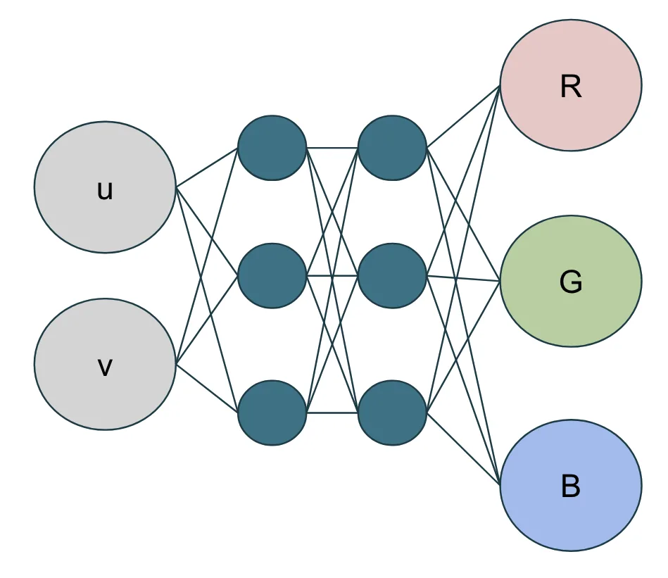
Continuing with our focus on texture representation as an example, we can create a simple network that takes texture UV coordinates as input and generates RGB color output. With just nine parameters (six weights and three biases), we can represent what would otherwise require 200,000 floats in a traditional texture.

For this specific network, we’ll use the hyperbolic tangent (tanh()) as our activation function—a simple and common choice for neural networks. To train it, we use an optimization step built into our framework. We’ll see that our Python NetworkParameters class has an optimize() method; this method is a wrapper that calls the adamOptimize() function in our Slang module. This adamOptimize() function is where the actual optimization algorithm is implemented and executed on the GPU—in this case, a basic version of the popular Adam optimizer.

Here’s a basic implementation of a neural network in Slang:

import slangpy;


// Simple activation function (tanh)
[Differentiable]
float activation(float x)
{
    return tanh(x);
}

// Simple Adam optimizer for a single parameter
void adamOptimize(
    inout float primal,      // The parameter to optimize
    inout float grad,        // The gradient
    inout float m_prev,      // First moment (running average of gradient)
    inout float v_prev,      // Second moment (running average of squared gradient)
    float learning_rate,     // Learning rate
    int iteration)           // Current iteration number
{
    const float ADAM_BETA_1 = 0.9;
    const float ADAM_BETA_2 = 0.999;
    const float ADAM_EPSILON = 1e-8;

    // Update first and second moments
    float m = ADAM_BETA_1 * m_prev + (1.0 - ADAM_BETA_1) * grad;
    float v = ADAM_BETA_2 * v_prev + (1.0 - ADAM_BETA_2) * (grad * grad);
    
    m_prev = m;
    v_prev = v;

    // Bias correction
    float mHat = m / (1.0f - pow(ADAM_BETA_1, iteration));
    float vHat = v / (1.0f - pow(ADAM_BETA_2, iteration));

    // Update parameter
    primal -= learning_rate * (mHat / (sqrt(vHat) + ADAM_EPSILON));
    
    // Reset gradient
    grad = 0;
}

// Network parameters with automatic differentiation support
struct NetworkParameters<int Inputs, int Outputs>
{
    RWTensor<float, 1> biases;
    RWTensor<float, 2> weights;

    AtomicTensor<float, 1> biases_grad;
    AtomicTensor<float, 2> weights_grad;

    [Differentiable]
    float get_bias(int neuron)
    {
        return biases.get({neuron});
    }
    [Differentiable]

And here’s how to set up and train the network in Python:

import slangpy as spy
import numpy as np
import pathlib

# Create device and load the Slang module
device = spy.create_device(
    include_paths=[
        pathlib.Path(__file__).parent.absolute(),
    ]
)
module = spy.Module.load_from_file(device, "example.slang")


# Python wrapper for the Slang NetworkParameters struct
class NetworkParameters(spy.InstanceList):
    def __init__(self, inputs: int, outputs: int):
        super().__init__(module[f"NetworkParameters<{inputs},{outputs}>"])
        self.inputs = inputs
        self.outputs = outputs

        # Biases and weights for the layer.
        self.biases = spy.Tensor.from_numpy(device, 
            np.zeros(outputs).astype('float32'))
        self.weights = spy.Tensor.from_numpy(device, 
            np.random.uniform(-0.5, 0.5, (outputs, inputs)).astype('float32'))

        # Gradients for the biases and weights.
        self.biases_grad = spy.Tensor.zeros_like(self.biases)
        self.weights_grad = spy.Tensor.zeros_like(self.weights)

        # Temp data for Adam optimizer.
        self.m_biases = spy.Tensor.zeros_like(self.biases)
        self.m_weights = spy.Tensor.zeros_like(self.weights)
        self.v_biases = spy.Tensor.zeros_like(self.biases)
        self.v_weights = spy.Tensor.zeros_like(self.weights)

    # Calls the Slang 'optimize' function for biases and weights
    def optimize(self, learning_rate: float, optimize_counter: int):
        module.adamOptimize(self.biases, self.biases_grad, self.m_biases,
            self.v_biases, learning_rate, optimize_counter)
        module.adamOptimize(self.weights, self.weights_grad, self.m_weights,
            self.v_weights, learning_rate, optimize_counter)

# Create network parameters for a layer with 2 inputs and 3 outputs
params = NetworkParameters(2, 3)

print(f"Created NetworkParameters with {params.inputs} inputs and {params.outputs} outputs")
print(f"Biases shape: {params.biases.shape}")
print(f"Weights shape: {params.weights.shape}")
print(f"Initial weights:\n{params.weights.to_numpy()}")

For more complex networks, you can easily add multiple layers:

// Multi-layer network for more complex texture generation
struct Network {
    NetworkParameters<2, 32>  layer0;
    NetworkParameters<32, 32> layer1;
    NetworkParameters<32, 3>  layer2;

    [Differentiable]
    float3 eval(no_diff float2 uv)
    {
        float inputs[2] = {uv.x, uv.y};
        float output0[32] = layer0.forward(inputs);
        [ForceUnroll]
        for (int i = 0; i < 32; ++i)
            output0[i] = activation(output0[i]);

        float output1[32] = layer1.forward(output0);
        [ForceUnroll]
        for (int i = 0; i < 32; ++i)
            output1[i] = activation(output1[i]);

        float output2[3] = layer2.forward(output1);
        [ForceUnroll]
        for (int i = 0; i < 3; ++i)
            output2[i] = activation(output2[i]);

        return float3(output2[0], output2[1], output2[2]);
    }
}

The beauty of this approach is that the same autodiff infrastructure that worked for simple parameter optimization now works for neural network training. The compiler automatically generates the gradients for the entire network, making it easy to train complex texture generation models.

Key techniques for better results

Small networks require careful engineering to work well. The techniques that work best depend on your specific application—what helps with texture generation may not be optimal for material evaluation or lighting calculations. Here are some key techniques that can dramatically improve results for the texture example we’ve been looking at:

• Activation functions: One commonly used activation function in machine learning is the rectified linear unit (ReLU), which simply emits any positive input unchanged, and outputs zero for any negative input. While computationally efficient and effective for many neural shading tasks, it can create piecewise linear outputs due to their thresholding at zero. This can lead to visible triangular patterns in 2D texture applications. Smoother activations, like exponential functions, often provide better visual quality for texture generation. The choice of activation function depends on the specific use case.

// Some alternative activation functions
[Differentiable]
float3 smoothActivation(float3 x) {
    return exp(x); // Exponential activation for smoother output
}

[Differentiable
float3 leakyReLU(float3 x) {
    return max(0.1 * x, x); // Leaky ReLU prevents dead neurons
}

• Leaky ReLU: When ReLU outputs zero (for negative inputs), the gradient becomes zero, as well. This means that during backpropagation, no updates are sent back to the weights that feed into that neuron. If a neuron consistently receives negative inputs during training, it can become permanently “dead”—outputting zero and never learning. This is particularly problematic in small networks where losing even a few neurons can hurt performance. Leaky ReLU instead outputs a small negative value (typically 0.01 times the input), ensuring the gradient is never exactly zero, so the neuron continues learning even when its input is negative. The small negative slope keeps the neuron “alive” and responsive to gradient updates.
• Frequency encoding: Instead of directly feeding raw UV coordinates to a neural network, we first pass them through sines and cosines of different frequencies. This improves quality without increasing computational cost. Neural networks struggle to learn high-frequency (fine details, sharp transitions) patterns from low-dimensional inputs. By encoding coordinates as [sin(2πu), cos(2πu), sin(2πv), cos(2πv)], we provide the network with multiple frequency components. This allows it to learn both low-frequency (smooth) and high-frequency patterns, which are especially beneficial for spatial inputs like UV coordinates. It’s less useful for non-spatial inputs where frequency content isn’t a primary concern.

// Frequency encoding for better neural texture representation
float4 encodeUV(float2 uv) {
    float4 encoded;
    encoded.x = sin(uv.x * 2.0 * 3.14159);
    encoded.y = cos(uv.x * 2.0 * 3.14159);
    encoded.z = sin(uv.y * 2.0 * 3.14159);
    encoded.w = cos(uv.y * 2.0 * 3.14159);
    return encoded;
}

// Enhanced network with frequency encoding
[Differentiable]
float3 evaluateNetworkWithEncoding(NeuralNetwork net, float2 uv) {
    float4 encoded = encodeUV(uv);
    // Now use 4D input instead of 2D
    float3 output = float3(0.0, 0.0, 0.0);
    for (int i = 0; i < 3; i++) {
        output[i] = net.biases[i];
        for (int j = 0; j < 4; j++) {
            output[i] += net.weights[i * 4 + j] * encoded[j];
        }
    }
    return smoothActivation(output);
}

How cooperative vectors accelerate hardware 

Modern GPUs have dedicated Tensor Cores that can efficiently compute matrix multiplications. However, using Tensor Cores requires cooperative execution where all threads operate together to compute a matrix multiplication.

Cooperative vectors provide a convenient way to access this hardware. They enable you to write shader code as normal matrix-vector multiplication, and the compiler automatically maps it to Tensor Core hardware without requiring explicit packing or uniform control flow.

Here’s how to use cooperative vectors for neural network acceleration:

struct FeedForwardLayer<int InputSize, int OutputSize>
{
    ByteAddressBuffer weights;
    uint weightsOffset;
    ByteAddressBuffer biases;
    uint biasesOffset;

    CoopVec<float, OutputSize> eval(CoopVec<float, InputSize> input)
    {
        let output = coopVecMatMulAdd<float, OutputSize>(
            input, CoopVecComponentType.Float32, // input and format
            weights, weightsOffset, CoopVecComponentType.Float32, // weights and format
            biases, biasesOffset, CoopVecComponentType.Float32, // biases and format
            CoopVecMatrixLayout.ColumnMajor, // matrix layout
            false, // is matrix transposed
            sizeof(float) * InputSize); // matrix stride


        return max(CoopVec<float, OutputSize>(0.0f), output); // ReLU activation
    }
}

Real-world applications: What can you build?

The techniques we’ve covered form the foundation for many exciting applications in neural shading. Here are some of the most promising areas:

Neural texture compression (NTC)

Neural texture compression represents one of the most practical applications of neural shading. Traditional block compression formats like BC1 and BC7 have fundamental limitations, but NTC can deliver much higher quality at similar compression rates or much better compression at similar quality levels.

The key insight is to use a small neural network as a decoder, fed with low-precision latent textures and positional encoding. This approach offers several advantages:

• Variable bit rates: Using a variable number of latent textures with low bit depth gives a wide range of encoding bit rates (0.5 to 20 bits per pixel).
• Independent decoding: Each pixel can be decoded independently, enabling direct sampling in shaders.
• No hallucinations: Unlike large image-generation models, small networks trained from scratch for each texture don’t produce entirely generated artifacts like extra fingers.

For implementation details and examples, see the NVIDIA neural texture compression library.

Neural materials

Neural materials represent another powerful application—learning complex, layered materials and distilling them into small networks that run significantly faster than the original shader code.

The approach involves training a network to take light direction, viewing direction, and latent codes as input, and to provide material color as output. For spatial variation, we train a texture of latent codes that we feed as additional input.

The key innovation is using an encoder network during training that translates the original material textures into latent textures, then baking the result for runtime use. This approach scales to very high texture resolutions (4K and beyond) without the convergence issues of per-texel optimization.

Beyond textures and materials

The principles of neural shading extend far beyond these examples. You can apply similar techniques to:

• Lighting calculations: Approximate complex lighting models with fast neural approximations.
• Post-processing effects: Learn optimal tone mapping, color grading, or stylization effects.
• Geometry processing: Generate or modify geometry procedurally with neural networks.
• Animation: Create smooth interpolations or procedural animations.
• Procedural generation: Generate content algorithmically with learned patterns.
• De-noising for ray tracing: Reduce noise in ray-traced images.
• Animation compression: Compress animation data efficiently with learned representations.
• Mesh simplification: Simplify 3D meshes while preserving detail in the final appearance.

The key is identifying where you have expensive computations or complex relationships that could benefit from neural approximation.

The future: Why neural shading matters

Neural shading represents more than just a new technique—it’s a fundamental shift in how we think about real-time graphics. By making shaders trainable, we open up new possibilities:

• Quality-performance tradeoffs: Networks can be smoothly adjusted for different quality levels, enabling natural LOD systems.
• Extensible features: Additional learned components can be easily added to networks for tasks like importance sampling or filtering.
• Platform flexibility: The same neural assets can work across different hardware capabilities, using inference and sample on capable hardware and transcoding on less-capable platforms.

The key to success is building up a mental toolbox of optimization techniques and debugging skills specific to neural shading. Just as with any new technology, there’s a learning curve, but the rewards are substantial.

Getting started: your next steps

The neural shading ecosystem is maturing rapidly. Here are the key tools and libraries you need to get started:

• Slang: The core shading language with autodiff support
• SlangPy: Python interface for rapid prototyping
• RTX Neural Shaders SDK: Comprehensive library for neural network inference and training
• Cooperative vector examples: End-to-end examples showing hardware acceleration

To get started fast with Slang and autodiff, you can try it out in your browser at the Slang Playground. For comprehensive resources and tools, explore the NVIDIA RTX Kit, which includes support for neural shading technologies. To dive deeper into the concepts covered in this guide, watch the neural shading course NVIDIA presented at SIGGRAPH.

At the Graphics Programming Conference (GPC) next week, be sure to check out our Neural Shading for Real-Time Graphics and Path Tracing in Doom the Dark Ages sessions.

The technology is ready for production use today. Whether you’re working on texture compression, material systems, or entirely new applications, neural shading provides a powerful new tool for achieving higher quality and better performance in real-time graphics.

See our full list of game developer resources here and follow us to stay up-to-date with the latest NVIDIA game development news: 

• Join the NVIDIA Developer Program (select gaming as your industry)
• Follow us on social: X, LinkedIn, Facebook, and YouTube
• Join our Discord community