
Julia is a high-level programming language for mathematical computing that is as easy to use as Python, but as fast as C. The language has been created with performance in mind, and combines careful language design with a sophisticated LLVM-based compiler [Bezanson et al. 2017].
Julia is already well regarded for programming multicore CPUs and large parallel computing systems, but recent developments make the language suited for GPU computing as well. The performance possibilities of GPUs can be democratized by providing more high-level tools that are easy to use by a large community of applied mathematicians and machine learning programmers. In this blog post, I will focus on native GPU programming with a Julia package that enhances the Julia compiler with native PTX code generation capabilities: CUDAnative.jl.
Existing GPU-Accelerated Julia Packages
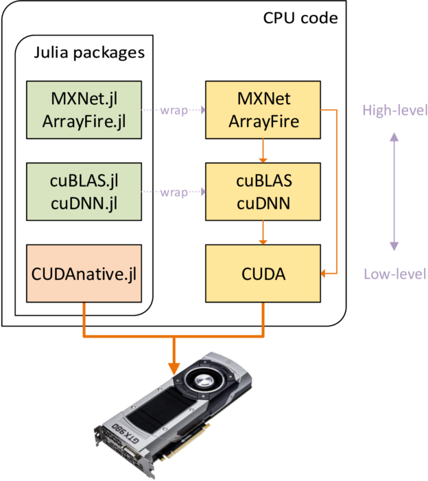
The Julia package ecosystem already contains quite a few GPU-related packages, targeting different levels of abstraction as Figure 1 shows. At the highest abstraction level, domain-specific packages like MXNet.jl and TensorFlow.jl can transparently use the GPUs in your system. More generic development is possible with ArrayFire.jl, and if you need a specialized CUDA implementation of a linear algebra or deep neural network algorithm you can use vendor-specific packages like cuBLAS.jl or cuDNN.jl. All these packages are essentially wrappers around native libraries, making use of Julia’s foreign function interfaces (FFI) to call into the library’s API with minimal overhead. For more information, check out the JuliaGPU GitHub organization which hosts many of these packages.
What’s missing from this list is the lowest abstraction level, where you can write kernels and manage execution like you would in CUDA C++. Such flexibility might be required to implement or optimize algorithms that cannot be cleanly expressed using the abstractions from existing packages. This is where CUDAnative.jl comes in.
Native GPU Programming with CUDAnative.jl
The CUDAnative.jl package adds native GPU programming capabilities to the Julia programming language. Used together with the CUDAdrv.jl or CUDArt.jl package for interfacing with the CUDA driver and runtime libraries, respectively, you can now do low-level CUDA development in Julia without an external language or compiler. As an introductory example, the following listing shows how to compute the sum of two vectors.
using CUDAdrv, CUDAnative

function kernel_vadd(a, b, c)
    i = threadIdx().x
    c[i] = a[i] + b[i]
    return
end

# generate some data
len = 512
a = rand(Int, len)
b = rand(Int, len)

# allocate & upload to the GPU
d_a = CuArray(a)
d_b = CuArray(b)
d_c = similar(d_a)

# execute and fetch results
@cuda (1,len) kernel_vadd(d_a, d_b, d_c)
c = Array(d_c)
The real workhorse of this example is the @cuda macro, which generates specialized code for compiling the kernel function to GPU assembly, uploading it to the driver, and preparing the execution environment. Together with Julia’s just-in-time (JIT) compiler, this results in a very efficient kernel launch sequence, avoiding runtime overhead typically associated with dynamic languages. The generated code is also specific to the types of the arguments; Calling the same kernel with differently typed arguments “just works”.
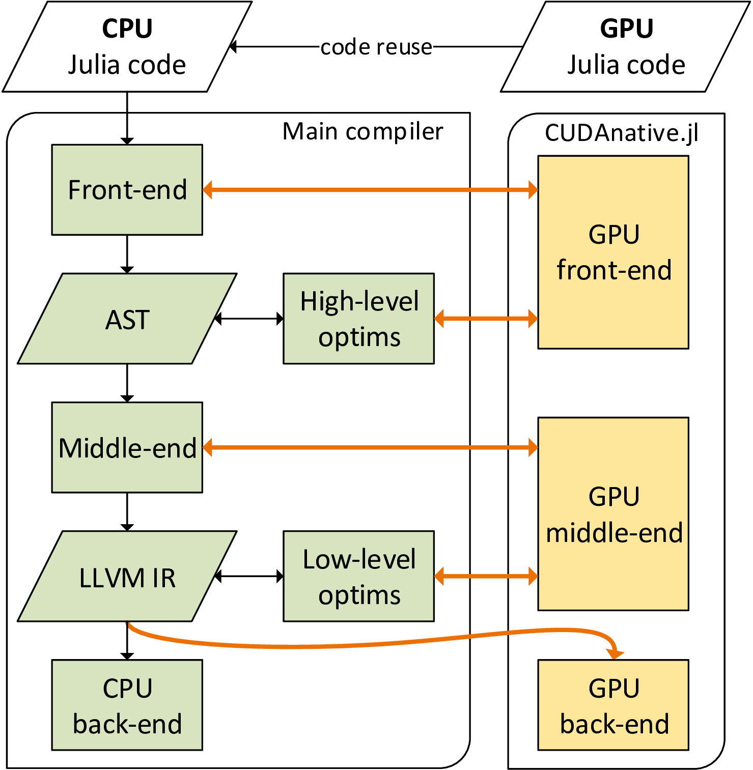
The design of the Julia GPU compiler avoids providing a custom toolchain to compile (a GPU-compatible subset of) Julia source code to GPU assembly. Instead, as you can see in Figure 2, it integrates with the existing Julia compiler as much as possible. Only the final step of generating machine code is fully specific to the GPU support package.
Reusing the Julia compiler has many advantages. For one, it keeps the hardware support packages tiny: CUDAnative.jl is only 1300 lines of code. CUDAnative.jl also avoids multiple independent language implementations, which often result in slightly different semantics. That means you use the Julia language for GPU functions just as you would for CPU code. You can use dynamically-typed multimethods, metaprogramming, arbitrary types and objects, and more. Of course, there are still some incompatibilities and limitations; for example, there is not yet a Julia GPU runtime library or garbage collector. But these aren’t structural limitations, and the Julia team is continuously working towards covering more of the language and libraries.
Example: Parallel Reduction
For a more interesting example, let’s have a look at parallel reduction. Parallel reduction is a cooperative parallel algorithm (discussed on this blog before) commonly used to compute a sum or other single value from a sequence of input values. The Julia code I show here is part of the CUDAnative examples and is too long to include in full, so let’s zoom in on some details instead.
The following snippet shows the innermost device function responsible for reducing within a warp using GPU shuffle instructions (slightly simplified for readability).
function reduce_warp(op, val)
    offset = CUDAnative.warpsize() ÷ 2
    while offset > 0
        val = op(val, shfl_down_sync(val, offset))
        offset ÷= 2  # truncating division
    end
    return val
end
This function takes two arguments, a reduction operator function and a value to reduce. The Julia compiler generates specialized code based on the types of these arguments, not only avoiding run-time type checks but completely inlining the function argument. This can be seen in the code listing below, showing the PTX code generated for this function when called with the + operator and a 32-bit integer as arguments (similar tools exist to inspect the typed AST, LLVM IR, or even GPU SASS assembly code).
julia> CUDAnative.@code_ptx reduce_warp(+, Int32(42))

.visible .func  (.param .b32 func_retval0) reduce_warp(
        .param .b32 param_0
)
{
        .reg .pred      %p<3>;
        .reg .s32       %r<17>;

        ld.param.u32    %r16, [param_0];
        mov.u32         %r8, WARP_SZ;
        shr.u32         %r15, %r8, 1;
        setp.eq.s32     %p1, %r15, 0;
        @%p1 bra        LBB0_3;
        mov.u32         %r12, 31;
        mov.u32         %r13, -1;
LBB0_2:
        shfl.sync.down.b32 %r9, %r16, %r15, %r12, %r13;
        add.s32         %r16, %r9, %r16;
        shr.u32         %r15, %r15, 1;
        setp.eq.s32     %p2, %r15, 0;
        @%p2 bra        LBB0_3;
        bra.uni         LBB0_2;
LBB0_3:
        st.param.b32    [func_retval0+0], %r16;
        ret;
}
Function specialization is automatic, and empowers much of the generic code in Julia’s standard library. In the case of this example, it results in clean and compact PTX code very similar to the code generated by nvcc.
Performance
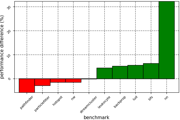
The big question, of course, is whether this high-level programming comes at a cost. As I’ve shown with the parallel reduction, CUDAnative.jl generates efficient PTX code for small functions, but how does that hold up for real-life applications? To assess this, the Julia team has been porting the Rodinia benchmark suite for heterogeneous accelerators to Julia. Because porting such applications is a large effort, we’ve focused on the 10 smallest benchmarks.
The chart in Figure 3 compares the performance of the original CUDA C++ implementations of these benchmarks against our Julia ports. The Julia versions are almost verbatim ports, that is, with no algorithmic changes and not introducing high-level concepts, in order to assess compiler performance differences as exactly as possible. As you can see, using Julia for GPU computing doesn’t suffer from any broad performance penalty. The only outlier is the nn benchmark, which performs significantly better with CUDAnative.jl due to slightly better register usage. On average, the CUDAnative.jl ports perform identical to statically compiled CUDA C++ (the difference is ~2% in favor of CUDAnative.jl, excluding nn). This is in part because of the work by Google on the NVPTX LLVM back-end.
NVIDIA Tools
CUDAnative.jl also aims to be compatible with existing tools from the CUDA toolkit. For example, it generates the necessary line number information for the NVIDIA Visual Profiler to work as expected, and wraps relevant API functions to have more fine-grained control. The line number information also enables accurate backtraces in combination with tools like cuda-memcheck:
$ cuda-memcheck julia examples/oob.jl
========= CUDA-MEMCHECK
========= Invalid __global__ write of size 4
=========     at 0x00000148 in examples/oob.jl:14:julia_memset_66041
=========     by thread (10,0,0) in block (0,0,0)
=========     Address 0x1020b000028 is out of bounds
Full debug information is not supported by the LLVM NVPTX back-end yet, so cuda-gdb will not work yet.
High-Level Programming
A native equivalent to CUDA C++ is only where the fun begins. Julia’s combination of dynamic language semantics, a specializing JIT compiler and first-class metaprogramming makes it possible to create really powerful high-level abstractions that are hard to realize in other dynamic languages, and downright impossible with statically compiled code. Thanks to CUDAnative.jl, it is now possible to create such abstractions for GPU programming, without sacrificing performance.
For example, the CuArrays.jl package combines the performance of CUBLAS.jl and flexibility of CUDAnative.jl to offer CUDA-accelerated arrays that behave just like any other array in Julia. It builds on Julia’s support for higher-order functions, which are automatically specialized: Calling map or broadcast on a CuArray generates a kernel specialized on the operation and array type, much like the above reduce_warp example.
In addition, Julia has recently gained support for syntactic loop fusion, where chained vector operations are fused into a single broadcast. Copying the example from the introductory blogpost, say we have a function \(f(x) = 3x^2 + 5x + 2\) and we want to evaluate \(f(2x^2 + 6x^3 – sqrt(x))\) for a GPU array X, storing the result in-place in X. You can now do the following.
X = CuArray(...)
f(x) = 3x^2 + 5x + 2
X .= f.(2 .* X.^2 .+ 6 .* X.^3 .- sqrt.(X))
This entire computation will be fused into a single GPU kernel, with performance comparable to a hand-written equivalent! The code is also dynamically typed, and works equally well for CPU arrays or even distributed containers, as long as the relevant methods are implemented. This is known as duck typing, and makes it much more easy to implement truly generic code. We are actively working on implementing all required interfaces to use GPU arrays with packages like ForwardDiff.jl (automatic differentiation) or Knet.jl (deep learning).
Lastly, Julia features a strong foreign function interface for calling into other language environments. It empowers packages like Cxx.jl, a FFI for C++ that can parse headers and call functions accordingly. We are using that interface to create CUDAnativelib.jl for calling CUDA device libraries, some of which are shipped as templated C++ headers (eg. cuRAND).
Try it out!
Many of the packages listed at the top of this post are relatively mature, and support a wide range of platforms and Julia versions. CUDAnative.jl and its dependents are still a work-in-progress and do not offer the same level of compatibility yet. For example, we only support Linux and macOS, and require a source build of Julia. Head over to this blogpost for an overview of the (pretty easy) installation instructions, or just pull this docker image.
If you’re interested in using Julia for native GPU programming, please try out CUDAnative.jl and let us know how you like it, on Discourse, Slack, or the issue tracker. While we will continue to improve platform support and language compatibility, it’s good to have feedback on real users and use-cases.
References
[Bezanson et al. 2017] Julia: A fresh approach to numerical computing. Jeff Bezanson, Alan Edelman, Stefan Karpinski, Viral B. Shah. SIAM Review, vol. 59.